Improving Wavelength Calibration Accuracy Across the CCD

Learning Goals

The wavelength calibration accuracy of STIS CCD spectra is stable at the detector center, while significant offsets are present toward the CCD top and bottom edges and increase with time, as suggested in recent works: STIS ISR 2026-03 and STIS ISR 2026-04.

An update to CalSTIS has now been implemented to apply row-selected wavecal processing for observations taken with the E1/E2 pseudo-apertures, while preserving the standard procedure for nominal extractions, as explained in the May 2026 STAN.

However, the updated pipeline improves the wavelength calibration only for spectra extracted at the E1/E2 positions. Spectra extracted at other locations on the CCD other than E1/E2 or the center — for example when using POS-TARG offsets or when analyzing extended sources — may still require additional wavelength-shift corrections before scientific interpretation. For many G230MB E1 datasets, and for a few G230LB and G430M E1 datasets, the new wavelength calibration procedure returns incorrect SHIFTA1 (i.e., the dispersion-axis shift) values. This is due to a combination of low S/N and spurious features in the extracted wavecal spectra, which can affect the cross-correlation. This notebook illustrates a cross-correlation procedure that can be used to derive proper dispersion corrections in these cases.

In particular, you will learn how to perform row-selected cross-correlation on wavecal files to improve the wavelength calibration of spectra extracted at positions other than the nominal center or the E1/E2 pseudo-apertures, or in cases where the wavelength calibration fails. This will allow you to calculate the xoffset value(s) to use when extracting the science target spectra.

As an optional step, you will also learn how to manipulate and update the DISPTAB reference file for your specific datasets, in order to create correct 2D Spectral Images.

Table of Contents:

• Import Packages

• Configure Matplotlib

• Download Data

• Wavelength calibration on Wavecal

• Spectra Extraction

• Example 1 - Compact source at a position other than center and E1/E2

  • Read Wavecal Data

  • Read Lamp Reference File

  • Cross-correlation with Lamp Template To Determine Proper Shifts to Fix Offsets

  • Apply correction to wavecals to improve wavelength calibration accuracy

  • Final Plots

• Example 2 - Extended Source Across CCD Detector

  • Wavecal and Lamp Files

  • Cross-correlation with Lamp Template To Determine Proper Shifts to Fix Offsets

  • Apply correction to wavecals to improve wavelength calibration accuracy

  • Final Plots

• Conclusions

• Optional: update of the DISPTAB reference file

  • Correcting 2D Spectral Images (X2D/SX2)

  • Conclusions

Import Packages

# Import for: Managing system variables and file paths
import os
import shutil
from pathlib import Path
import stat

# Import for: Downloading necessary files
# (Not necessary if you choose to collect data from MAST)
from astroquery.mast import Observations

# Import for: Reading FITS files
from astropy.io import fits
from astropy.table import Table

# Import for: Calculation and Data Analysis
import numpy as np

# Import for: Aggregating and displaying tabulated data
import pandas as pd

# Import for: Smoothing data
from scipy.ndimage import gaussian_filter1d

# Import for: Model Fitting
from astropy.modeling import fitting
from astropy.modeling.models import Polynomial1D

# Import for: Performing cross-correlatoin
from scipy.signal import correlate
from scipy.signal import correlation_lags

# Import for: Operations on STIS Data
import stistools

# Import for: Plotting
import matplotlib
import matplotlib.pyplot as plt
from matplotlib.pyplot import cm

/home/runner/micromamba/envs/ci-env/lib/python3.12/site-packages/stsci/tools/nmpfit.py:8: UserWarning: NMPFIT is deprecated - stsci.tools v 3.5 is the last version to contain it.
  warnings.warn("NMPFIT is deprecated - stsci.tools v 3.5 is the last version to contain it.")
/home/runner/micromamba/envs/ci-env/lib/python3.12/site-packages/stsci/tools/gfit.py:18: UserWarning: GFIT is deprecated - stsci.tools v 3.4.12 is the last version to contain it.Use astropy.modeling instead.
  warnings.warn("GFIT is deprecated - stsci.tools v 3.4.12 is the last version to contain it."

The following tasks in the stistools package can be run with TEAL:
   basic2d      calstis     ocrreject     wavecal        x1d          x2d

# Gaussian full-width at half-max:
FWHM = 2 * np.sqrt(2 * np.log(2))  # ≈ 2.355

Configure Matplotlib Default Plotting Parameters

plt.rcParams['figure.figsize'] = (10, 15)
plt.rcParams['image.origin'] = 'lower'
plt.rcParams['lines.linewidth'] = 1
plt.rcParams['axes.titlesize'] = 'large'
plt.rcParams['axes.labelsize'] = 20
plt.rcParams['xtick.labelsize'] = 20
plt.rcParams['ytick.labelsize'] = 20
plt.rcParams['font.family'] = 'serif'
plt.rcParams['legend.facecolor'] = 'white'
plt.rcParams['legend.edgecolor'] = 'black'
plt.rcParams['legend.framealpha'] = 0.7
plt.rcParams['legend.fontsize'] = 15
plt.rcParams['legend.loc'] = 'upper right'
plt.rcParams['legend.frameon'] = True
plt.rcParams['legend.fancybox'] = True
plt.rcParams['legend.shadow'] = False
plt.rcParams['legend.numpoints'] = 1

Download Data

In this section, users should download the STIS datasets needed for their analysis from MAST.

This notebook uses the wavecal file for one G430L/c4300 dataset as an example, but the same procedure applies to all first-order gratings. Users can adapt the workflow by providing the appropriate obsid for their observations to download the corresponding wavecal file.

For G230MB data and a subset of G230LB and G430M, caution is required: wavecal spectra extracted near the CCD edges may have low signal-to-noise and few emission lines, which can affect the reliability of the cross-correlation offsets. This notebook can still be used to derive the offset at different detector positions and find the most appropriate correction.

# Path to the directory where you want to save the downloaded files and the results of the analysis

mypath = Path.cwd()
mypath

PosixPath('/home/runner/work/hst_notebooks/hst_notebooks/notebooks/STIS/e1_notebook')

# Modify this for your specific dataset (lower or upper case)
# These are a subset of tested datasets - here we look only at the wavecal files
obsid = 'oec63w010'  # g430l
# obsid = 'OFAJ23010'  # g430l
# obsid = 'OF8Q14010'  # g750l
# obsid = 'ODYH220D0'  # g750m
# obsid = 'o6ih10060'  # g430l
# obsid = 'OE3G010D0'  # g430m
# obsid = 'ofhcm1030'  # g230mb
# obsid = 'OF8B02020'  # g230lb

# Search dataset with the given obsid
obs_table = Observations.query_criteria(obs_id=obsid)

# Get a list of files assiciated with that target
products = Observations.get_product_list(obs_table)

# Filter product types to only wavecal files:
products = products[products['productSubGroupDescription'].filled() == 'WAV']

# Download FITS files
result = Observations.download_products(products, download_dir=mypath)

result

INFO: Found cached file /home/runner/work/hst_notebooks/hst_notebooks/notebooks/STIS/e1_notebook/mastDownload/HST/oec63w010/oec63w010_wav.fits with expected size 2260800. [astroquery.query]

Table length=1

Local Path	Status	Message	URL
str118	str8	object	object
/home/runner/work/hst_notebooks/hst_notebooks/notebooks/STIS/e1_notebook/mastDownload/HST/oec63w010/oec63w010_wav.fits	COMPLETE	None	None

Copy wavecal observations to dedicated directory:

def copy_files(source_file, destination_path):
    """Copy file to the destination path.

    Construct the destination path by joining the destination directory and the base
    name of the source file.
    """
    destination_file = os.path.join(destination_path, os.path.basename(source_file))
    shutil.copy(source_file, destination_file)
    print(f"File copied: {source_file} to {destination_file}")

Locate our wavecal:

wavfile = mypath / 'mastDownload' / 'HST' / obsid / f'{obsid}_wav.fits'
wavfile

PosixPath('/home/runner/work/hst_notebooks/hst_notebooks/notebooks/STIS/e1_notebook/mastDownload/HST/oec63w010/oec63w010_wav.fits')

copy_files(wavfile, destination_path=mypath)

File copied: /home/runner/work/hst_notebooks/hst_notebooks/notebooks/STIS/e1_notebook/mastDownload/HST/oec63w010/oec63w010_wav.fits to /home/runner/work/hst_notebooks/hst_notebooks/notebooks/STIS/e1_notebook/oec63w010_wav.fits

Explore Wavecal Data

wavfile = mypath / f'{obsid}_wav.fits'
hdr0 = fits.getheader(wavfile, ext=0)

print(f"target   = {hdr0['TARGNAME']}")
print(f"aperture = {hdr0['PROPAPER']}")
print(f"grating  = {hdr0['OPT_ELEM']}")
print(f"cenwave  = {hdr0['CENWAVE']}")
print(f"lamp   = {hdr0['SCLAMP']}")
print(f"date   = {hdr0['TDATEOBS']}")

grating = hdr0['OPT_ELEM']
cenwave = hdr0['CENWAVE']
lamp = hdr0['SCLAMP']

target   = WAVELINE
aperture = 52X0.1E1
grating  = G430L
cenwave  = 4300
lamp   = LINE
date   = 2020-12-12

Next, use the Calibration Reference Data System (CRDS) command line tools to update and download the reference files.

https://hst-crds.stsci.edu/

https://hst-crds.stsci.edu/docs/cmdline_bestrefs/

crds_path = os.path.expanduser("~") + "/crds_cache"
os.environ["CRDS_PATH"] = crds_path
os.environ["CRDS_SERVER_URL"] = "https://hst-crds.stsci.edu"
os.environ["oref"] = os.path.join(crds_path, "references/hst/oref/")

!crds bestrefs --update-bestrefs --sync-references=1 --files {obsid}_wav.fits

CRDS - INFO -  No comparison context or source comparison requested.

CRDS - INFO -  ===> Processing oec63w010_wav.fits

CRDS - INFO -  0 errors
CRDS - INFO -  0 warnings
CRDS - INFO -  2 infos

rawfile = f"{obsid}_wav.fits"

with fits.open(rawfile) as hdul:
    hdr = hdul[0].header

ref_keys = [
    "BIASFILE", "DARKFILE", "PFLTFILE", "LFLTFILE",
    "APERTAB", "SPTRCTAB", "DISPTAB", "INANGTAB", "LAMPTAB"
]

oref = os.environ["oref"]

for key in ref_keys:
    val = hdr.get(key)
    if val is None or val == "N/A":
        print(f"{key:8s} = {val}")
        continue

    if val.startswith("oref$"):
        path = val.replace("oref$", oref)
    else:
        path = val

    print(f"{key:8s} = {val:25s} exists={os.path.exists(path)}")
    if not os.path.exists(path):
        print("   missing path:", path)

BIASFILE = oref$5162002no_bia.fits   exists=True
DARKFILE = oref$5162002do_drk.fits   exists=True
PFLTFILE = oref$x6417094o_pfl.fits   exists=True
LFLTFILE = oref$pcc2026jo_lfl.fits   exists=True
APERTAB  = oref$y2r1559to_apt.fits   exists=True
SPTRCTAB = oref$qa31608go_1dt.fits   exists=True
DISPTAB  = oref$l2j0137to_dsp.fits   exists=True
INANGTAB = oref$h5s11397o_iac.fits   exists=True
LAMPTAB  = oref$l421050oo_lmp.fits   exists=True

Calibrate Wavecals

The function below calibrates the wavecal data as if they were science data.

In particular, CalSTIS ≥3.5.0 reads the PROPAPER keyword of the science raw file header for the wavelength calibration step to determine whether the E1/E2 wavelength-calibration optimization should be applied. Since here we want to derive wavelength corrections directly from the wavecal files at arbitrary CCD positions, we set PROPAPER to the nominal value so that the files are treated as nominal-center observations by CalSTIS.

def calibrate(wavefile, verbose=False):
    """Calibrate wavecal exposure as a science expsoure.

    1.  First, copy the _wav.fits file to _raw.fits to be used as a rawfile for wavecals.
    2.  Then, change the header keywords of the _raw file so that CalSTIS will extract it as science.
    3.  For this exercise, we also need to change the PROPAPER keyword to make sure that the wavecal
        is not processed as a science file taken at E1 (new CalSTIS ≥3.5.0 checks PROPAPER keyword in
        science data and here we are treating the wavecal as science).
    4.  Lastly, run CalSTIS.

    Parameters:
    -----------
    rawfile : str
        full path to the raw fits file

    verbose : bool
        print calstis stdout, default=False
    """
    wavefile = str(wavefile)  # allow pathlib.Path input types

    rawfile = wavefile.replace('_wav.fits', '_raw.fits')
    shutil.copy(wavefile, rawfile)

    # Set header keywords to process as science
    with fits.open(rawfile, mode='update') as f:
        f[0].header['WAVECAL'] = os.path.basename(wavefile)
        f[0].header['FLUXCORR'] = 'OMIT'
        f[0].header['WAVECORR'] = 'PERFORM'

        # Remove 'E1' if it is in PROPAPER:
        f[0].header['PROPAPER'] = f[0].header['PROPAPER'].replace('E1', '')

        f[1].header['ASN_MTYP'] = 'SCIENCE'

    # Redirect standard out text:
    trailer = '' if verbose else '/dev/null'

    res = stistools.calstis.calstis(rawfile, trailer=trailer)

    assert res == 0, 'calstis errored in call to "calibrate()"'

calibrate(wavfile)

This step provides us with a wavelength-calibrated wavecal file.

Move input and product files to tidy up:

# Make a destination directory if it does not yet exist:
wavecal_calibrated = mypath / 'wavecal_calibrated'
wavecal_calibrated.mkdir(parents=True, exist_ok=True)

# move files to destination
for filetype in ['flt', 'wav', 'raw', 'x2d']:
    for filename in mypath.glob(f"{obsid}_{filetype}.fits"):
        print(f"Moving {filename}")
        os.replace(filename, os.path.join(wavecal_calibrated, os.path.basename(filename)))

Moving /home/runner/work/hst_notebooks/hst_notebooks/notebooks/STIS/e1_notebook/oec63w010_flt.fits
Moving /home/runner/work/hst_notebooks/hst_notebooks/notebooks/STIS/e1_notebook/oec63w010_wav.fits
Moving /home/runner/work/hst_notebooks/hst_notebooks/notebooks/STIS/e1_notebook/oec63w010_raw.fits
Moving /home/runner/work/hst_notebooks/hst_notebooks/notebooks/STIS/e1_notebook/oec63w010_x2d.fits

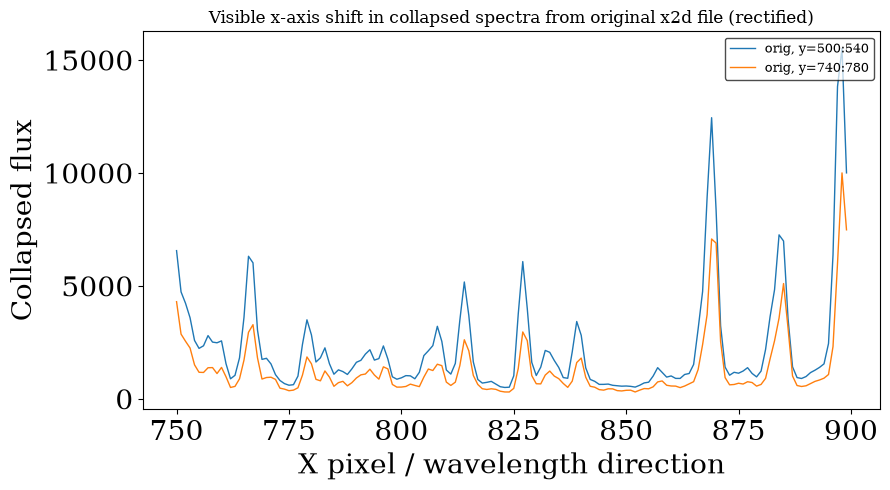
The plot below shows how in the X1D file obtained with the pipeline a spectrum at the edge is shifted with respect to a spectrum extracted at the center.

x2_orig = fits.getdata(wavecal_calibrated / f"{obsid}_x2d.fits", ext=1)

xrange = slice(750, 900)

yranges = [
    slice(500, 540),
    slice(740, 780),
]

x = np.arange(x2_orig.shape[1])[xrange]

fig, ax = plt.subplots(figsize=(9, 5))

for yrange in yranges:
    prof = np.nansum(x2_orig[yrange, xrange], axis=0)

    line, = ax.plot(
        x,
        prof,
        label=f'orig, y={yrange.start}:{yrange.stop}'
    )

ax.set_xlabel('X pixel / wavelength direction')
ax.set_ylabel('Collapsed flux')
ax.set_title('Visible x-axis shift in collapsed spectra from original x2d file (rectified)')
ax.legend(fontsize=9)
fig.tight_layout()
plt.savefig(mypath / f'x2d_collapsed_spectra_orig_{grating}_{cenwave}_{lamp}.png', dpi=300)

Extract spectra at desired Y-location and calculate correction factors

The functions below use stistools.x1d.x1d to extract spectra from the calibrated wavecal flt files. See details about x1d here:
https://spacetelescope.github.io/hst_notebooks/notebooks/STIS/extraction/1D_Extraction.html

The workflow is:

• Extract a reference spectrum at the nominal position (center = 512)

• For compact sources, extract a spectrum at the source position on the CCD

• For extended sources, extract spectra at multiple positions across the CCD

def extract(fltname, center, size, xoffset=0, verbose=False):
    """Use the x1d task to extract the final spectrum.

    Extraction of spectra, centered at column "center" (1-indexed),
    with extraction box of size "size".

    Parameters
    ----------
    fltname : str or pathlib.Path
        full path to the flt FITS file

    center : float
        extraction Y-location (1-indexed) for mid-detector X-location

    size : int
        extraction size in pixels

    xoffset : float
        offset in X

    Returns
    -------
    str : output filename
    """
    # Put additional string into output filename if an xoffset is specified:
    corr = '' if (xoffset == 0) else '_corr'

    fltname = str(fltname)  # allow pathlib.Path input types
    rootname = os.path.basename(fltname).replace('_flt.fits', '')
    outname = f"{rootname}{corr}_{center!s}_x1d.fits"

    # Redirect standard out text:
    trailer = '' if verbose else '/dev/null'

    if np.abs(xoffset) < 10:
        xoffset = xoffset
    else:
        xoffset = 0

    res = stistools.x1d.x1d(
        fltname,
        backcorr="omit",
        ctecorr="omit",
        dispcorr="perform",
        helcorr="omit",
        fluxcorr="omit",
        a2center=center,
        maxsrch=0,
        extrsize=size,
        xoffset=xoffset,
        output=outname,
        trailer=trailer)

    print(res)
    assert res == 0, 'stistools.x1d.x1d() returned an error'

    return outname

Example #1: Compact source at a position other than center and E1/E2

In the example below, spectra are extracted at the nominal center (512) and slightly below the E1 position (E1~900; here we extract at 750).

The value 750 can be replaced with any other CCD position corresponding to the location where you want to extract your source.

fltfile = wavecal_calibrated / f"{obsid}_flt.fits"

extract(fltfile, 512, size=40)
extract(fltfile, 750, size=40)

0
0

'oec63w010_750_x1d.fits'

# Make a destination directory if it does not yet exist:
wavecal_extracted = mypath / 'wavecal_extracted'
wavecal_extracted.mkdir(parents=True, exist_ok=True)

for filename in mypath.glob(f"{obsid}_*_x1d.fits"):
    os.replace(filename, os.path.join(wavecal_extracted, os.path.basename(filename)))

Here we compare the spectra extracted from the wavecal file to the lamp template to perform a cross-correlation and derive the wavelength offset.

Read wavecal spectra and print some statistics:

# Data at position 512:
wlspec_C = wavecal_extracted / f"{obsid}_512_x1d.fits"
with fits.open(wlspec_C) as f:
    wl_wlspec_C = f[1].data['WAVELENGTH'][0]
    flux_wlspec_C = f[1].data['NET'][0]

wl_mean_plate_scale_C = (wl_wlspec_C[1:] - wl_wlspec_C[:-1]).mean()

print('\nAt Y=512:')
minwl, maxwl = np.nanmin(wl_wlspec_C), np.nanmax(wl_wlspec_C)
print(f"Wavelength range of data:  {minwl:.0f} - {maxwl:.0f} Å")
print(f"Mean plate scale:  {wl_mean_plate_scale_C:.5f} Å/pix")

# Data at position 750:
wlspec_E = wavecal_extracted / f"{obsid}_750_x1d.fits"
with fits.open(wlspec_E) as f:
    wl_wlspec_E = f[1].data['WAVELENGTH'][0]  # index at order 0 (only first-order is present here)
    flux_wlspec_E = f[1].data['NET'][0]

wl_mean_plate_scale_E = (wl_wlspec_E[1:] - wl_wlspec_E[:-1]).mean()

print('\nAt Y=750:')
print(f"Wavelength range of data:  {np.nanmin(wl_wlspec_E):.0f} - {np.nanmax(wl_wlspec_E):.0f} Å")
print(f"Mean plate scale:  {wl_mean_plate_scale_E:.5f} Å/pix")

At Y=512:
Wavelength range of data:  2898 - 5707 Å
Mean plate scale:  2.74645 Å/pix

At Y=750:
Wavelength range of data:  2894 - 5703 Å
Mean plate scale:  2.74604 Å/pix

Read Lamp Reference File

The lamp reference file should be downloaded and added in folder from here:
https://hst-crds.stsci.edu/unchecked_get/references/hst/l421050oo_lmp.fits

This spectrum is the one used as reference for the wavelength calibration. Here we will degrade it to the spectra resolution of our wavecal spectra and interpolate it on the same x-range, before performing the cross-correlation.

Read lamptab file and select the same wavelength range as wavecal data:

lamp_ref = Table.read(os.path.join(crds_path, 'references/hst/stis/', 'l421050oo_lmp.fits'))

# Keep only the SCLAMP='ANY' row, discarding the 'PRISM' row:
lamp_ref = lamp_ref[[x.strip() == 'ANY' for x in lamp_ref['SCLAMP']]]

lamp_ref

Table length=1

SCLAMP	LAMPSET	OPT_ELEM	NELEM	WAVELENGTH	FLUX	PEDIGREE	DESCRIP
	mA			Angstroms	counts
bytes6	bytes6	bytes8	int32	float64[300000]	float32[300000]	bytes67	bytes67
ANY	ANY	ANY	256814	1131.82 .. 0	0.166667 .. 0	GROUND	Ground Cal for non-PRISM, PT lamp 10 mA

wl_lamp = lamp_ref['WAVELENGTH'][0].data
flux_lamp = lamp_ref['FLUX'][0].data

# Trim the lamp wavelengths down to the wavecal's range:
w = (wl_lamp > minwl) & (wl_lamp < maxwl)
lamp_wl_sel = wl_lamp[w]
lamp_flux_sel = flux_lamp[w]

mean_plate_scale_lamp_sel = (lamp_wl_sel[1:] - lamp_wl_sel[:-1]).mean()
print(f"Lamp Mean Plate Scale Lamp:  {mean_plate_scale_lamp_sel:.5f}")

Lamp Mean Plate Scale Lamp:  0.09527

Degrade Lamp Spectrum to wavecal data spectral resolution:

# Degrade to E1 resolution
degraded_lamp_flux_E = gaussian_filter1d(lamp_flux_sel, wl_mean_plate_scale_E / FWHM / mean_plate_scale_lamp_sel)

# Degrade to C resolution
degraded_lamp_flux_C = gaussian_filter1d(lamp_flux_sel, wl_mean_plate_scale_C / FWHM / mean_plate_scale_lamp_sel)

print(f"Degradation kernel sigma for E1:  {wl_mean_plate_scale_E / FWHM / mean_plate_scale_lamp_sel:.2f} pixels")
print(f"Degradation kernel sigma for C:  {wl_mean_plate_scale_C / FWHM / mean_plate_scale_lamp_sel:.2f} pixels")

Degradation kernel sigma for E1:  12.24 pixels
Degradation kernel sigma for C:  12.24 pixels

Interpolate degraded lamp spectrum to wavelength points in the wavecal data:

flux_lamp_interp_E = np.interp(wl_wlspec_E, lamp_wl_sel, degraded_lamp_flux_E)
flux_lamp_interp_C = np.interp(wl_wlspec_C, lamp_wl_sel, degraded_lamp_flux_C)

Plot normalized spectra to compare between wavecal spectrum extracted at detector center and lamp spectrum:

# Normalize spectra
flux_C_norm = (flux_wlspec_C - np.nanmedian(flux_wlspec_C)) / np.nanstd(flux_wlspec_C)
flux_E_norm = (flux_wlspec_E - np.nanmedian(flux_wlspec_E)) / np.nanstd(flux_wlspec_E)

lamp_orig_norm = (lamp_flux_sel - np.nanmedian(lamp_flux_sel)) / np.nanstd(lamp_flux_sel)
lamp_interp_norm = (flux_lamp_interp_C - np.nanmedian(flux_lamp_interp_C)) / np.nanstd(flux_lamp_interp_C)

# Find peak from interpolated lamp spectrum
ipeak = np.nanargmax(lamp_interp_norm)
wl_peak = wl_wlspec_C[ipeak]

# Define wavelength range
dw = 50  # Angstrom
wl_min = wl_peak - dw
wl_max = wl_peak + dw

plt.figure(figsize=(15, 8))

plt.plot(
    wl_wlspec_C,
    flux_C_norm,
    color='magenta', lw=2, linestyle='dashed',
    label='Extracted Wavecal Spectrum - C'
)

plt.plot(
    wl_wlspec_E,
    flux_E_norm,
    color='magenta', lw=2, linestyle='dotted', 
    label='Extracted Wavecal Spectrum - E1')

plt.plot(
    lamp_wl_sel,
    lamp_orig_norm,
    color='lightgray', lw=0.5,
    label='Original Lamp Spectrum'
)

plt.plot(
    wl_wlspec_C,
    lamp_interp_norm,
    color='gray', lw=2,
    label='Interpolated Lamp Spectrum'
)

plt.xlim(wl_min, wl_max)
plt.ylim(-0.5, 13)

plt.title(
    'Extracted Wavecal Spectrum, Lamp Spectrum, and Interpolated Lamp Spectrum',
    size=15
)
plt.legend()
plt.xlabel('Wavelength (Å)')
plt.ylabel('Normalized Intensity')

plt.savefig(
    mypath / f'extracted_wavecal_spectra_and_lamp_{grating}_{cenwave}_{lamp}.png',
    dpi=300,
    bbox_inches='tight'
)
plt.show()

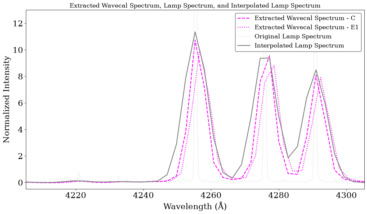
The plot above shows that the wavecal extracted at the center of the detector and the lamp template are well aligned, as expected for the nominal position.

However, there is a clear wavelength shift between the degraded lamp template and the extracted spectrum.

Cross-correlation with Lamp Template To Determine Proper Shifts to Fix Offsets

The cross-correlation function cross_correlate is taken from cross-correlation notebook here: https://github.com/spacetelescope/STIS-Notebooks

Lag and Cross-Correlation Coefficient
The lag is the displacement (in pixels) in the lagged spectrum. If the lag is 0, the spectra are aligned and not shifted.

The cross-correlation coefficient encodes how similar two spectra are. The cross-correlation coefficient takes values from -1 to 1: if it’s positive, the 2 spectra are positively correlated; if it’s negative, the 2 spectra are anti-correlated.

The cross-correlation algorithm shifts one of the input spectra according the the lag values and computes the cross-correlation coefficient for each lag. Then we take the sub-pixel-shift lag with the maximum cross-correlation coefficient and compute the corresponding displacement in wavelength space.

Normalization of the input spectra is required to ensure the cross-correlation coefficient is in the [-1, 1] range.

def cross_correlate(shifted_flux, ref_flux):
    '''Evaluate the cross-correlation of two arrays vs shift.
    '''
    if len(shifted_flux) != len(ref_flux):
        raise ValueError('Arrays must be same size')

    # normalize inputs
    shifted_flux = shifted_flux - shifted_flux.mean()
    shifted_flux /= shifted_flux.std()
    ref_flux = ref_flux - ref_flux.mean()
    ref_flux /= ref_flux.std()

    # centered at the median of len(a)
    lag = correlation_lags(len(shifted_flux), len(ref_flux), mode="same")
    # find the cross-correlation coefficient
    cc = correlate(shifted_flux, ref_flux, mode="same") / float(len(ref_flux))

    return lag, cc

def apply_crosscorr(shifted_flux, ref_flux, mean_plate_scale, plot=True, ax=None, note=''):
    '''Calculate the cross-correlation between two arrays and fit the peak.
    '''
    # cross-correlate inputs
    lag, cc = cross_correlate(shifted_flux, ref_flux)

    # fit a quadratic near the peak to find the pixel shift
    fitter = fitting.LinearLSQFitter()

    # get the 3 points nearest the peak
    width = 3
    low, hi = np.argmax(cc) - width // 2, np.argmax(cc) + width // 2 + 1
    fit = fitter(Polynomial1D(degree=2), x=lag[low:hi], y=cc[low:hi])
    x_c = np.arange(-5, 5, 0.01)           

    shift_px = -fit.parameters[1] / (2. * fit.parameters[2])  # pixels
    shift_wl = shift_px * mean_plate_scale  # Å

    if plot:
        if ax is None:
            fig, ax = plt.subplots(nrows=1, ncols=1)
            fig.set_size_inches(12, 5)
            fig.tight_layout()
            fig.subplots_adjust(wspace=0.2, hspace=0.1, top=0.88)

        ax.plot(lag, cc, ".-", label="cross-correlation coefficient")
        ax.plot(x_c, fit(x_c), alpha=0.5, label="fitted quadratic curve")
        ax.plot([shift_px, shift_px], [0, 1], alpha=0.5, label="quadratic curve maximum")
        ax.set_ylabel("CC Coeff.")
        ax.set_ylim(0, 1)
        ax.set_xlim(-17, 17)
        ax.grid(True, alpha=0.2)
        note += '; ' if note else ''
        ax.set_title(f"{note}Pixel Shift: {shift_px:.2f} px, Wavelength Shift: {shift_wl:.2f} Å", size=15)
        ax.legend(fontsize=10)
        ax.axhline(0, linestyle='dashed', c='k', alpha=0.05)
        ax.set_xlabel("Lag (pix)")
        plt.savefig(mypath / f'cross_correlation_{note.replace("; ", "")}_{grating}_{cenwave}_{lamp}.png', dpi=300)

    return (shift_px, shift_wl)

Apply cross-correlation between the lamp template and the two spectra extracted at center and other location to retrieve shift in pixels and in Angstroms.

fig, axes = plt.subplots(2, 1)
fig.set_size_inches(12, 5*len(axes))
fig.tight_layout(pad=5.0)

shift_px_C, shift_wl_C = apply_crosscorr(
    flux_wlspec_C[5:-5], flux_lamp_interp_C[5:-5], wl_mean_plate_scale_C,
    plot=True, ax=axes[0], note='Y=512')

shift_px_E, shift_wl_E = apply_crosscorr(
    flux_wlspec_E[5:-5], flux_lamp_interp_E[5:-5], wl_mean_plate_scale_E,
    plot=True, ax=axes[1], note='Y=750')

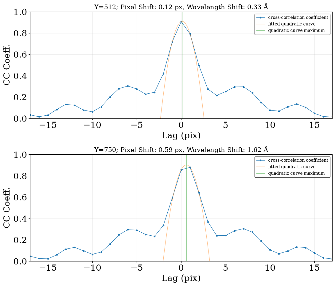
If the derived shift is unusually large (i.e., several pixels) and the plot above does not show a good fit, the cross-correlation likely failed.

This can happen if the extracted wavecal spectrum at a given position has insufficient S/N, or if spurious features, such as cosmic-ray residuals, dominate the cross-correlation. In this case, users can try increasing the extraction size (this example uses EXTRSIZE = 40), choosing a slightly different A2CENTER (still close to the desired position), or selecting a wavelength subrange with clear emission lines while avoiding spurious features before repeating the cross-correlation.

print(f"Pixel Shift for Y=512: {shift_px_C:+5.2f} px, Wavelength Shift for Y=512: {shift_wl_C:+5.2f} Å")
print(f"Pixel Shift for Y=750: {shift_px_E:+5.2f} px, Wavelength Shift for Y=750: {shift_wl_E:+5.2f} Å")

Pixel Shift for Y=512: +0.12 px, Wavelength Shift for Y=512: +0.33 Å
Pixel Shift for Y=750: +0.59 px, Wavelength Shift for Y=750: +1.62 Å

From the output shown above, the spectrum extracted at the detector center is already well aligned with the lamp template.

In contrast, the spectrum extracted near the detector edge shows a significant shift, exceeding the nominal wavelength calibration accuracy of about 0.2-0.3 pixels.

Apply correction to improve wavelength calibration accuracy

This example is shown for the wavecal data, but the same procedure applies to the science spectrum extracted at the same position.

The pixel shift derived in the cross-correlation step is considered in the spectra extraction using the xoffset parameter.

outname = extract(fltfile, center=750, size=40, xoffset=shift_px_E, verbose=False)
outname

0

'oec63w010_corr_750_x1d.fits'

os.replace(mypath / outname, wavecal_extracted / outname)

Read new extracted spectrum:

# Data at position 750 corrected
wlspec_E_corr = wavecal_extracted / outname

with fits.open(wlspec_E_corr) as f:
    wl_wlspec_E_corr = f[1].data['WAVELENGTH'][0]
    flux_wlspec_E_corr = f[1].data['NET'][0]

Plot Cross-Correlation Corrected Edge Spectrum

# Normalize spectra
flux_C_norm = (flux_wlspec_C - np.nanmedian(flux_wlspec_C)) / np.nanstd(flux_wlspec_C)
flux_E_norm = (flux_wlspec_E - np.nanmedian(flux_wlspec_E)) / np.nanstd(flux_wlspec_E)
flux_E_corr_norm = (flux_wlspec_E_corr - np.nanmedian(flux_wlspec_E_corr)) / np.nanstd(flux_wlspec_E_corr)

# Define automatic wavelength range
dw = 50  # Angstrom
wl_min = wl_peak - dw
wl_max = wl_peak + dw

fig, axes = plt.subplots(2, 1, sharex=True, sharey=True)
fig.set_size_inches(12, 6 * len(axes))

for ax in axes:
    ax.plot(
        wl_wlspec_C,
        flux_C_norm,
        color='orangered',
        lw=2,
        linestyle='dashed',
        label='Center Spectrum'
    )

axes[0].plot(
    wl_wlspec_E,
    flux_E_norm,
    color='forestgreen',
    lw=2,
    linestyle='solid',
    label='Edge Spectrum'
)

axes[1].plot(
    wl_wlspec_E_corr,
    flux_E_corr_norm,
    color='forestgreen',
    lw=2,
    linestyle='solid',
    label='Edge Spectrum - Corrected'
)

axes[1].set_xlabel('Wavelength (Å)')
axes[0].set_xlim(wl_min, wl_max)
axes[0].set_ylim(-1, 13)

for ax in axes:
    ax.set_ylabel('Normalized Flux')
    ax.grid(alpha=0.5)

handles, labels = axes[0].get_legend_handles_labels()
fig.legend(
    handles,
    labels,
    loc='center left',
    bbox_to_anchor=(1.0, 0.5),
    title='Spectrum',
    fontsize=14,
    title_fontsize=14
)

axes[0].set_title('Extracted Wavecal Spectra at Selected Rows — Original')
axes[1].set_title('Extracted Wavecal Spectra at Selected Rows — After Cross-Correlation Correction')

fig.tight_layout()
plt.savefig(
    mypath / f'extracted_wavecal_spectra_before_after_cross_corr_{grating}_{cenwave}_{lamp}.png',
    dpi=300,
    bbox_inches='tight'
)
plt.show()

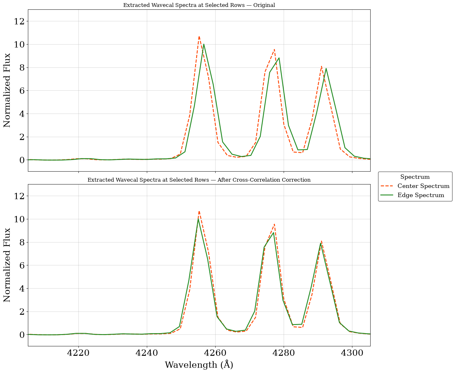
As shown in the bottom panel, applying the xoffset parameter during the extraction step brings the spectrum extracted near the edge of the CCD into agreement with the spectrum extracted at the detector center.

This example illustrates how to derive the required xoffset value (in pixels). Users can then re-extract their science spectra from the corresponding FLT or CRJ files at the desired detector position by providing the appropriate xoffset in the extraction step.

Example #2: Extended Source Across CCD Detector

In this case, we likely need to extract multiple spectra at different positions across the CCD.

To do this, we extract spectra from the wavecal FLT file at 33 different positions corresponding to the A2CENTER locations defined in the STIS reference files. Users can change the list_center array here below with alternate values.

# a2center is defined at these Y-positions in the DSP table:
list_centers = np.array([
    1, 33, 65, 97, 129, 161, 193, 225, 257, 289, 321,
    353, 385, 417, 449, 481, 513, 545, 577, 609, 641, 673,
    705, 737, 769, 801, 833, 865, 897, 929, 961, 993, 1024,])

len(list_centers)

33

fltfile = wavecal_calibrated / f"{obsid}_flt.fits"
fltfile

PosixPath('/home/runner/work/hst_notebooks/hst_notebooks/notebooks/STIS/e1_notebook/wavecal_calibrated/oec63w010_flt.fits')

for list_center in list_centers:
    extract(fltfile, list_center, size=40)

0
0
0
0
0
0
0
0

0
0
0
0
0
0
0
0

0
0
0
0
0
0
0
0

0
0
0
0
0
0
0
0

0

# Make a destination directory if it does not yet exist:
wavecal_extracted_extended_source = mypath / 'wavecal_extracted_extended_source'
wavecal_extracted_extended_source.mkdir(parents=True, exist_ok=True)

# move to destination directory
for filename in mypath.glob(f"{obsid}_*_x1d.fits"):
    os.replace(filename, os.path.join(wavecal_extracted_extended_source, os.path.basename(filename)))

Wavecal and Lamp Files

As for case #1, here we compare the spectra extracted from the wavecal file with the lamp template to perform a cross-correlation and derive the wavelength offset to be applied to the science data.

Read the wavecal spectra to determine the mean plate scale vs Y:

df = pd.DataFrame(data={'list_center': list_centers, 'wlspec': '', 'Min Wl': -1., 'Max Wl': -1.})

for i, row in df.iterrows():
    df.loc[i, 'wlspec'] = f"{obsid}_{row['list_center']}_x1d.fits"
    wlspec = wavecal_extracted_extended_source / df.loc[i, 'wlspec']

    with fits.open(wlspec) as f:
        wl_wlspec = f[1].data['WAVELENGTH'].squeeze()
        flux_wlspec = f[1].data['NET'].squeeze()
        fluxerr_wlspec = f[1].data['NET_ERROR'].squeeze()

        df.loc[i, 'Min Wl'] = np.nanmin(wl_wlspec)
        df.loc[i, 'Max Wl'] = np.nanmax(wl_wlspec)
        df.loc[i, 'Mean Plate Scale'] = (wl_wlspec[1:] - wl_wlspec[0:-1]).mean()

df

	list_center	wlspec	Min Wl	Max Wl	Mean Plate Scale
0	1	oec63w010_1_x1d.fits	2904.097022	5710.387668	2.743197
1	33	oec63w010_33_x1d.fits	2904.059407	5710.726926	2.743566
2	65	oec63w010_65_x1d.fits	2903.951478	5710.973401	2.743912
3	97	oec63w010_97_x1d.fits	2903.777875	5711.131711	2.744236
4	129	oec63w010_129_x1d.fits	2903.543246	5711.206487	2.744539
5	161	oec63w010_161_x1d.fits	2903.252240	5711.202363	2.744819
6	193	oec63w010_193_x1d.fits	2902.909513	5711.123981	2.745078
7	225	oec63w010_225_x1d.fits	2902.519725	5710.975987	2.745314
8	257	oec63w010_257_x1d.fits	2902.087539	5710.763035	2.745528
9	289	oec63w010_289_x1d.fits	2901.617622	5710.489781	2.745721
10	321	oec63w010_321_x1d.fits	2901.114644	5710.160889	2.745891
11	353	oec63w010_353_x1d.fits	2900.583278	5709.781025	2.746039
12	385	oec63w010_385_x1d.fits	2900.028200	5709.354858	2.746165
13	417	oec63w010_417_x1d.fits	2899.454088	5708.887061	2.746269
14	449	oec63w010_449_x1d.fits	2898.865623	5708.382310	2.746351
15	481	oec63w010_481_x1d.fits	2898.267486	5707.845281	2.746410
16	513	oec63w010_513_x1d.fits	2897.664362	5707.280656	2.746448
17	545	oec63w010_545_x1d.fits	2897.060935	5706.693114	2.746464
18	577	oec63w010_577_x1d.fits	2896.461891	5706.087336	2.746457
19	609	oec63w010_609_x1d.fits	2895.871918	5705.468005	2.746428
20	641	oec63w010_641_x1d.fits	2895.295701	5704.839801	2.746377
21	673	oec63w010_673_x1d.fits	2894.737928	5704.207407	2.746304
22	705	oec63w010_705_x1d.fits	2894.203287	5703.575501	2.746209
23	737	oec63w010_737_x1d.fits	2893.696462	5702.948761	2.746092
24	769	oec63w010_769_x1d.fits	2893.222141	5702.331865	2.745953
25	801	oec63w010_801_x1d.fits	2892.785007	5701.729485	2.745791
26	833	oec63w010_833_x1d.fits	2892.389745	5701.146293	2.745608
27	865	oec63w010_865_x1d.fits	2892.041034	5700.586956	2.745402
28	897	oec63w010_897_x1d.fits	2891.743557	5700.056138	2.745174
29	929	oec63w010_929_x1d.fits	2891.501988	5699.558497	2.744923
30	961	oec63w010_961_x1d.fits	2891.321005	5699.098689	2.744651
31	993	oec63w010_993_x1d.fits	2891.205278	5698.681361	2.744356
32	1024	oec63w010_1024_x1d.fits	2891.159477	5698.311159	2.744039

Truncate the lamp spectrum range, degrade its resolution, and interpolate to the X1D file wavelength grid:
(Also perform a cross-correlation with a subset of the wavelengths to aid in the low-SNR regime - You can also inspect the lamp spectrum and decide an appropriate range.)

wmin_subset, wmax_subset = wl_min, wl_max

print(f'Sub-set wavelength range for cross-correlation: {wmin_subset:.0f} - {wmax_subset:.0f} Å')

Sub-set wavelength range for cross-correlation: 4205 - 4305 Å

for i, row in df.iterrows():
    # Truncate LAMPTAB range to full wavecal range:
    w = (wl_lamp > row['Min Wl']) & (wl_lamp < row['Max Wl'])

    # Alternatively, truncate LAMPTAB range to a subset of the wavecal range:
    #   This is more robust to noisy lamp spectra and could improve the cross-correlation.
    w_subset = (wl_wlspec > wmin_subset) & (wl_wlspec < wmax_subset)

    lamp_wl_sel = wl_lamp[w]

    degraded_lamp_flux = gaussian_filter1d(
        flux_lamp[w],
        row['Mean Plate Scale'] / FWHM / mean_plate_scale_lamp_sel)

    with fits.open(wavecal_extracted_extended_source / row['wlspec']) as f:
        # Interpolate to data wavelength grid:
        flux_lamp_interp = np.interp(
            f[1].data['WAVELENGTH'][0],
            lamp_wl_sel,
            degraded_lamp_flux)

        # Run the cross-correlation on most of the wavelengths (except edges):
        df.loc[i, 'shift_px'], df.loc[i, 'shift_wl'] = apply_crosscorr(
            f[1].data['NET'][0][5:-5],
            flux_lamp_interp[5:-5],
            row['Mean Plate Scale'],
            plot=False)

        # Run the cross-correlation on a smaller subset of wavelengths:
        df.loc[i, 'shift_px_subset'], df.loc[i, 'shift_wl_subset'] = apply_crosscorr(
            f[1].data['NET'][0][w_subset],
            flux_lamp_interp[w_subset],
            row['Mean Plate Scale'],
            plot=False)

df

	list_center	wlspec	Min Wl	Max Wl	Mean Plate Scale	shift_px	shift_wl	shift_px_subset	shift_wl_subset
0	1	oec63w010_1_x1d.fits	2904.097022	5710.387668	2.743197	-0.298235	-0.818116	-0.229905	-0.630674
1	33	oec63w010_33_x1d.fits	2904.059407	5710.726926	2.743566	-0.249142	-0.683536	-0.211385	-0.579947
2	65	oec63w010_65_x1d.fits	2903.951478	5710.973401	2.743912	-0.223562	-0.613433	-0.197162	-0.540995
3	97	oec63w010_97_x1d.fits	2903.777875	5711.131711	2.744236	-0.197621	-0.542318	-0.175986	-0.482947
4	129	oec63w010_129_x1d.fits	2903.543246	5711.206487	2.744539	-0.160596	-0.440761	-0.151077	-0.414636
5	161	oec63w010_161_x1d.fits	2903.252240	5711.202363	2.744819	-0.148537	-0.407708	-0.130216	-0.357418
6	193	oec63w010_193_x1d.fits	2902.909513	5711.123981	2.745078	-0.121962	-0.334796	-0.095967	-0.263436
7	225	oec63w010_225_x1d.fits	2902.519725	5710.975987	2.745314	-0.094326	-0.258955	-0.049946	-0.137116
8	257	oec63w010_257_x1d.fits	2902.087539	5710.763035	2.745528	-0.055911	-0.153505	-0.003185	-0.008744
9	289	oec63w010_289_x1d.fits	2901.617622	5710.489781	2.745721	0.008798	0.024157	0.068812	0.188939
10	321	oec63w010_321_x1d.fits	2901.114644	5710.160889	2.745891	0.015805	0.043399	0.077407	0.212552
11	353	oec63w010_353_x1d.fits	2900.583278	5709.781025	2.746039	0.036494	0.100215	0.096193	0.264151
12	385	oec63w010_385_x1d.fits	2900.028200	5709.354858	2.746165	0.053221	0.146154	0.109324	0.300222
13	417	oec63w010_417_x1d.fits	2899.454088	5708.887061	2.746269	0.081548	0.223952	0.129214	0.354855
14	449	oec63w010_449_x1d.fits	2898.865623	5708.382310	2.746351	0.093520	0.256838	0.135342	0.371698
15	481	oec63w010_481_x1d.fits	2898.267486	5707.845281	2.746410	0.107074	0.294068	0.142535	0.391459
16	513	oec63w010_513_x1d.fits	2897.664362	5707.280656	2.746448	0.121137	0.332695	0.150512	0.413375
17	545	oec63w010_545_x1d.fits	2897.060935	5706.693114	2.746464	0.131194	0.360319	0.153954	0.422828
18	577	oec63w010_577_x1d.fits	2896.461891	5706.087336	2.746457	0.168450	0.462642	0.186422	0.512000
19	609	oec63w010_609_x1d.fits	2895.871918	5705.468005	2.746428	0.203857	0.559879	0.219529	0.602920
20	641	oec63w010_641_x1d.fits	2895.295701	5704.839801	2.746377	0.255663	0.702148	0.268266	0.736759
21	673	oec63w010_673_x1d.fits	2894.737928	5704.207407	2.746304	0.310806	0.853568	0.322239	0.884967
22	705	oec63w010_705_x1d.fits	2894.203287	5703.575501	2.746209	0.378315	1.038933	0.380288	1.044349
23	737	oec63w010_737_x1d.fits	2893.696462	5702.948761	2.746092	0.418483	1.149193	0.421675	1.157959
24	769	oec63w010_769_x1d.fits	2893.222141	5702.331865	2.745953	0.607850	1.669128	0.616426	1.692678
25	801	oec63w010_801_x1d.fits	2892.785007	5701.729485	2.745791	0.702847	1.929870	0.723354	1.986178
26	833	oec63w010_833_x1d.fits	2892.389745	5701.146293	2.745608	0.847068	2.325715	0.864540	2.373687
27	865	oec63w010_865_x1d.fits	2892.041034	5700.586956	2.745402	1.010085	2.773090	1.029026	2.825091
28	897	oec63w010_897_x1d.fits	2891.743557	5700.056138	2.745174	1.230637	3.378313	1.281637	3.518315
29	929	oec63w010_929_x1d.fits	2891.501988	5699.558497	2.744923	1.545374	4.241932	1.608206	4.414402
30	961	oec63w010_961_x1d.fits	2891.321005	5699.098689	2.744651	1.814563	4.980343	1.872012	5.138018
31	993	oec63w010_993_x1d.fits	2891.205278	5698.681361	2.744356	2.095809	5.751646	2.168040	5.949873
32	1024	oec63w010_1024_x1d.fits	2891.159477	5698.311159	2.744039	2.333825	6.404108	2.392668	6.565575

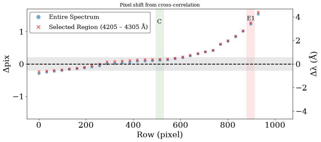
Plot results, assuming the average plate scale:

fig, ax = plt.subplots(1, 1)
fig.set_size_inches(12, 5)

ax.plot(df['list_center'], df['shift_px'], 'o', alpha=0.6, label='Entire Spectrum')
ax.plot(df['list_center'], df['shift_px_subset'], 'rx', mew=2, alpha=0.6, label=f'Selected Region ({wmin_subset:.0f} – {wmax_subset:.0f} Å)')

# Highlight C and E1 extraction regions:
ax.axvspan(880, 912, alpha=0.1, color='red')
ax.annotate(xy=(881, 1.35), text='E1', color='k', size=15)
ax.axvspan(496, 528, alpha=0.1, color='green')
ax.annotate(xy=(501, 1.25), text='C', color='k', size=15)

ax.axhspan(-0.2, 0.2, alpha=0.5, color='lightgray')
ax.axhline(0, linestyle='dashed', color='k', lw=2)

ax.set_ylim(-1.7, 1.7)
# ax.set_ylim(-0.7, 2.6)
# Plot the right-side Y-axis in wavelength:
ax_right = ax.twinx()
ax_right.set_ylim(np.array(ax.get_ylim()) * df['Mean Plate Scale'].mean())
ax_right.set_ylabel('Δλ (Å)')

ax.set_title('Pixel shift from cross-correlation')
ax.set_xlabel('Row (pixel)')
ax.set_ylabel('Δpix')
ax.legend(loc='best', markerscale=1.5)

plt.savefig(mypath / f'cross_correlation_pixel_shifts_{grating}_{cenwave}_{lamp}.png', dpi=300, bbox_inches='tight')

Plot the normalized spectra:

# Normalize interpolated lamp and find peak
lamp_interp_norm = (
    flux_lamp_interp_C - np.nanmedian(flux_lamp_interp_C)
) / np.nanstd(flux_lamp_interp_C)

ipeak = np.nanargmax(lamp_interp_norm)
wl_peak = wl_wlspec_C[ipeak]

dw = 50
wl_min = wl_peak - dw
wl_max = wl_peak + dw

fig, ax = plt.subplots(1, 1)
fig.set_size_inches(14, 6)

for position, linestyle, color, idx in zip(
    ['Lower Edge', 'Center', 'Upper Edge'],
    ['dashdot', 'dashed', 'dotted'],
    ['blue', 'magenta', 'red'],
    [4, 16, 30]
):

    with fits.open(wavecal_extracted_extended_source / df.loc[idx, 'wlspec']) as f:
        wl = f[1].data['WAVELENGTH'].squeeze()
        net = f[1].data['NET'].squeeze()

        net_norm = (net - np.nanmedian(net)) / np.nanstd(net)

        ax.plot(
            wl,
            net_norm,
            lw=2, alpha=0.8, color=color, linestyle=linestyle,
            label=f'Extracted Wavecal Spectrum at {position}'
        )

lamp_norm = (flux_lamp - np.nanmedian(flux_lamp)) / np.nanstd(flux_lamp)

ax.plot(
    wl_lamp,
    lamp_norm,
    lw=0.7, color='lightgray',
    label='Original Lamp Spectrum'
)

ax.plot(
    wl_wlspec_C,
    lamp_interp_norm,
    color='gray', lw=2,
    label='Interpolated Lamp Spectrum'
)

ax.set_xlim(wl_min, wl_max)
ax.set_ylim(-0.5, 13)

ax.legend(loc='best', fontsize=12)
ax.set_title(
    'Extracted Wavecal Spectra, Lamp Spectrum, and Interpolated Lamp Spectrum',
    size=15
)
ax.set_xlabel('Wavelength (Å)')
ax.set_ylabel('Normalized Net Counts')

# plt.xlim(4240, wl_max)
plt.savefig(
    mypath / f'extracted_wavecal_spectra_and_lamp_all_{grating}_{cenwave}_{lamp}.png',
    dpi=300,
    bbox_inches='tight'
)
plt.show()

Cross-correlation with Lamp Template To Determine Proper Shifts to Fix Offsets

Cross-correlation exactly as for Case #1.

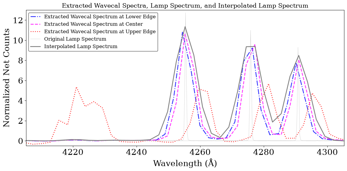
From these plots, users can assess the magnitude of the wavelength shifts across the CCD, which should be accounted for before extracting spectra of spatially extended targets.

Apply correction to improve wavelength calibration accuracy

This example is shown for the wavecal data, but the same procedure applies to the science spectrum extracted at the same position.

The pixel shift derived in the cross-correlation step is considered in the spectral extraction using the xoffset parameter.

for i, row in df.iterrows():
    extract(fltfile, row['list_center'], size=32, xoffset=row['shift_px_subset'])

0
0
0
0
0
0
0
0
0

0
0
0
0
0
0
0
0
0

0
0
0
0
0
0
0
0
0

0
0
0
0
0
0

# Make a destination directory if it does not yet exist:
wavecal_extracted_extended_source = mypath / 'wavecal_extracted_extended_source'
wavecal_extracted_extended_source.mkdir(parents=True, exist_ok=True)

# move files to destination
for filename in mypath.glob(f'{obsid}_corr_*_x1d.fits'):
    os.replace(filename, os.path.join(wavecal_extracted_extended_source, os.path.basename(filename)))

Plot Cross-Correlation Corrected Spectra at All Positions on Detector

offset_corrected = pd.DataFrame(data={'list_center': list_centers})
offset_corrected['wlspec'] = offset_corrected['list_center'].apply(lambda x: f'{obsid}_corr_{x:.0f}_x1d.fits')
offset_corrected['wlspec_unshifted'] = offset_corrected['list_center'].apply(lambda x: f'{obsid}_{x:.0f}_x1d.fits')
offset_corrected['offset'] = df['shift_px_subset']

fig, axes = plt.subplots(2, 1, figsize=(15, 15), sharex=True, sharey=True)
fig.subplots_adjust(hspace=0)

colors = cm.jet(np.linspace(0, 1, len(list_centers)))

for i, row in offset_corrected.iterrows():
    with (fits.open(wavecal_extracted_extended_source / row['wlspec']) as f_corr,
          fits.open(wavecal_extracted_extended_source / row['wlspec_unshifted']) as f_unshifted):

        wl_wlspec_corr = f_corr[1].data['WAVELENGTH'].squeeze()
        flux_wlspec_corr = f_corr[1].data['NET'].squeeze()
        fluxerr_wlspec_corr = f_corr[1].data['NET_ERROR'].squeeze()

        wl_wlspec_unshifted = f_unshifted[1].data['WAVELENGTH'].squeeze()
        flux_wlspec_unshifted = f_unshifted[1].data['NET'].squeeze()
        fluxerr_wlspec_unshifted = f_unshifted[1].data['NET_ERROR'].squeeze()

        axes[0].plot(
            wl_wlspec_unshifted,
            (flux_wlspec_unshifted - np.nanmedian(flux_wlspec_unshifted)) / np.nanstd(flux_wlspec_unshifted),
            color=colors[i], label=f"{row['list_center']:.0f}")

        axes[1].plot(
            wl_wlspec_corr,
            (flux_wlspec_corr - np.nanmedian(flux_wlspec_corr)) / np.nanstd(flux_wlspec_corr),
            color=colors[i], label=f"{row['list_center']:.0f}")

for ax in axes:
    ax.set_ylabel('Normalized Net Counts')
    ax.grid(alpha=0.5)
    ax.set_xlim(wl_min, wl_max)

axes[1].set_xlabel('Wavelength (Å)')
axes[0].set_ylim(-1, 12)

handles, labels = axes[0].get_legend_handles_labels()
fig.legend(handles, labels,
           loc='center left',
           bbox_to_anchor=(0.9, 0.5),
           title='Row number',
           fontsize=14,
           title_fontsize=14)

fig.suptitle('Extracted Wavecal Spectra At Selected Rows Before and After Cross-Correlation Correction',
             size=14, y=0.895)
plt.savefig(mypath / f'extracted_wavecal_spectra_before_after_cross_corr_2_{grating}_{cenwave}_{lamp}.png', dpi=300, bbox_inches='tight')

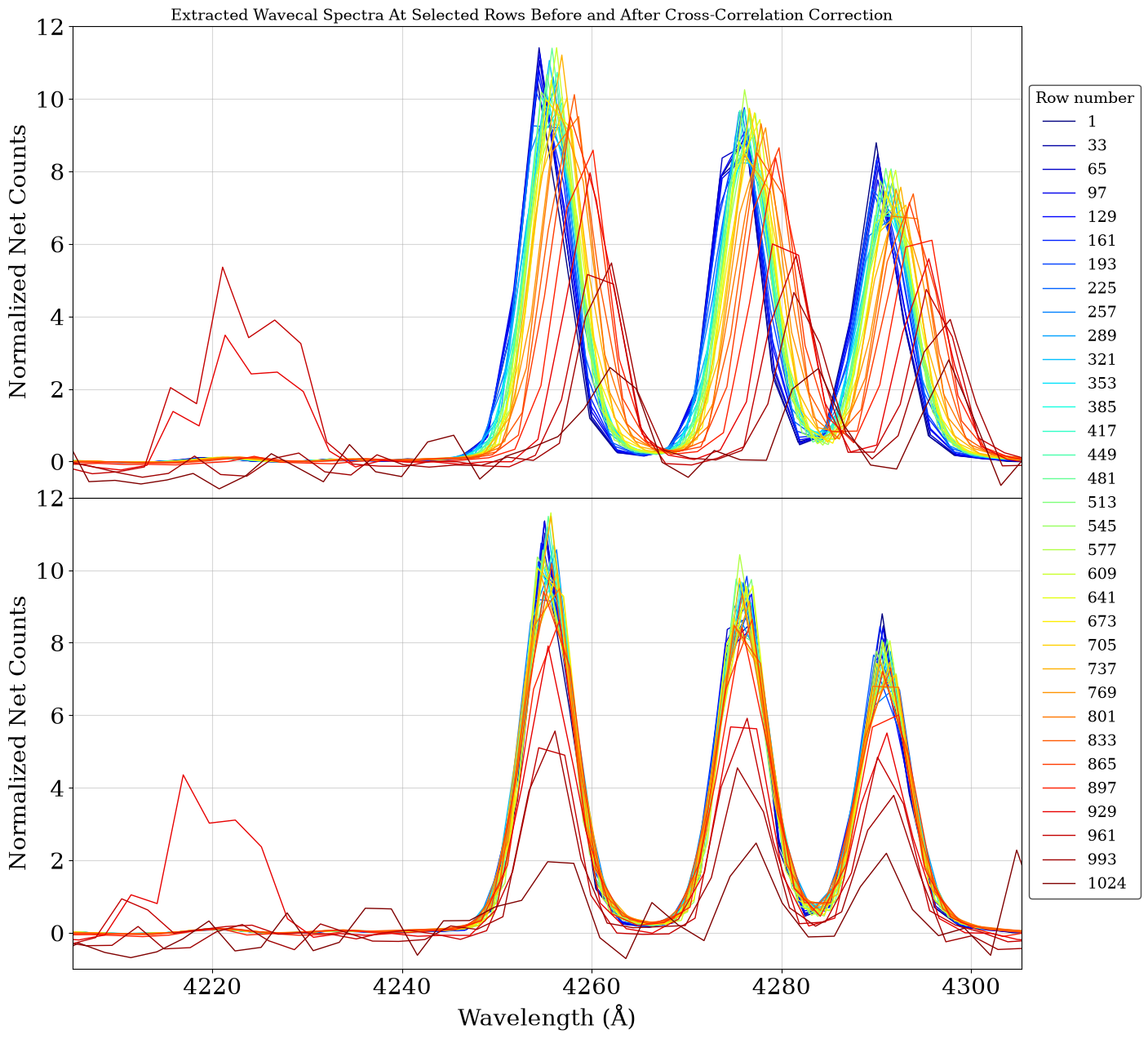
As shown in the bottom panel of the previous figure, applying the xoffset parameter during the extraction step brings the spectra extracted across the CCD into agreement with the spectrum extracted at the detector center.

Conclusions

This example illustrates how to derive the xoffset values (in pixels) required to align spectra extracted at different detector positions. The offsets can be measured from the wavecal observations as demonstrated here and then applied the same xoffsets during the extraction of the corresponding science spectra from the FLT or CRJ files.

Optional: update of the DISPTAB reference file

This optional step builds on Example #2 and should be run after completing it. It is needed to correct 2D spectral images intended for use with extended objects, and can be used to extract 1D spectra without using xoffset.

Correcting 2D Spectral Images (X2D/SX2)

Spectroscopic X2D and SX2 files are 2D spectral images that have been rectified. SX2 files combine multiple reads (either from REPEATOBS or CRSPLITs). Wavecal observations typically only take one read, but most science observations take multiple CRSPLITs in order to reject cosmic rays.

Here we show how to modify the DISPTAB to remove the residual wavelength shift vs Y-position found above for 1D spectra. By updating DISPTAB taking into account the shift calculated with the cross-correlation at different positions will be automatically included. Thus, there will be no need to specify xoffset when extracting spectra and it will be possible to re-create corrected X2D and SX2 files.

# Make a destination directory if it does not yet exist:
wavecal_2d_product = mypath / 'wavecal_2d_product'
wavecal_2d_product.mkdir(parents=True, exist_ok=True)

for filetype in ['wav', 'flt']:
    for filename in wavecal_calibrated.glob(f"{obsid}_{filetype}.fits"):
        print(f"Copying {filename}")
        shutil.copy(filename, wavecal_2d_product)

Copying /home/runner/work/hst_notebooks/hst_notebooks/notebooks/STIS/e1_notebook/wavecal_calibrated/oec63w010_wav.fits
Copying /home/runner/work/hst_notebooks/hst_notebooks/notebooks/STIS/e1_notebook/wavecal_calibrated/oec63w010_flt.fits

The Dispersion Relation Table (DISPTAB) encodes the inverse wavelength solution as a cubic function, with coefficients that vary with Y (A2CENTER) position. CalSTIS interpolates between these Y positions when applying the 2D correction.

The DSP reference file should be downloaded and added in folder from here:
https://hst-crds.stsci.edu/browse/l2j0137to_dsp.fits

disptab = os.path.join(crds_path, 'references/hst/stis/', 'l2j0137to_dsp.fits')
disp = Table.read(disptab, hdu=1)

# Filter to grating/cenwave:
disp = disp[[(x['OPT_ELEM'].strip() == hdr0['OPT_ELEM']) & (x['CENWAVE'] == hdr0['CENWAVE']) for x in disp]]
disp

Table length=33

OPT_ELEM	CENWAVE	SPORDER	REF_APER	A2CENTER	NCOEFF	COEFF	PEDIGREE	DESCRIP
	Angstrom			pix
bytes6	int16	int16	bytes7	float32	int16	float64[10]	bytes30	bytes28
G430L	4300	1	52X0.05	1	8	-1072.44 .. 0	INFLIGHT 27/02/1997 24/11/1999	Lindler Postlaunch, May 2000
G430L	4300	1	52X0.05	33	8	-1072.26 .. 0	INFLIGHT 27/02/1997 24/11/1999	Lindler Postlaunch, May 2000
G430L	4300	1	52X0.05	65	8	-1072.05 .. 0	INFLIGHT 27/02/1997 24/11/1999	Lindler Postlaunch, May 2000
G430L	4300	1	52X0.05	97	8	-1071.82 .. 0	INFLIGHT 27/02/1997 24/11/1999	Lindler Postlaunch, May 2000
G430L	4300	1	52X0.05	129	8	-1071.58 .. 0	INFLIGHT 27/02/1997 24/11/1999	Lindler Postlaunch, May 2000
G430L	4300	1	52X0.05	161	8	-1071.32 .. 0	INFLIGHT 27/02/1997 24/11/1999	Lindler Postlaunch, May 2000
G430L	4300	1	52X0.05	193	8	-1071.04 .. 0	INFLIGHT 27/02/1997 24/11/1999	Lindler Postlaunch, May 2000
G430L	4300	1	52X0.05	225	8	-1070.75 .. 0	INFLIGHT 27/02/1997 24/11/1999	Lindler Postlaunch, May 2000
G430L	4300	1	52X0.05	257	8	-1070.45 .. 0	INFLIGHT 27/02/1997 24/11/1999	Lindler Postlaunch, May 2000
...	...	...	...	...	...	...	...	...
G430L	4300	1	52X0.05	769	8	-1065.56 .. 0	INFLIGHT 27/02/1997 24/11/1999	Lindler Postlaunch, May 2000
G430L	4300	1	52X0.05	801	8	-1065.34 .. 0	INFLIGHT 27/02/1997 24/11/1999	Lindler Postlaunch, May 2000
G430L	4300	1	52X0.05	833	8	-1065.14 .. 0	INFLIGHT 27/02/1997 24/11/1999	Lindler Postlaunch, May 2000
G430L	4300	1	52X0.05	865	8	-1064.96 .. 0	INFLIGHT 27/02/1997 24/11/1999	Lindler Postlaunch, May 2000
G430L	4300	1	52X0.05	897	8	-1064.8 .. 0	INFLIGHT 27/02/1997 24/11/1999	Lindler Postlaunch, May 2000
G430L	4300	1	52X0.05	929	8	-1064.67 .. 0	INFLIGHT 27/02/1997 24/11/1999	Lindler Postlaunch, May 2000
G430L	4300	1	52X0.05	961	8	-1064.57 .. 0	INFLIGHT 27/02/1997 24/11/1999	Lindler Postlaunch, May 2000
G430L	4300	1	52X0.05	993	8	-1064.49 .. 0	INFLIGHT 27/02/1997 24/11/1999	Lindler Postlaunch, May 2000
G430L	4300	1	52X0.05	1024	8	-1064.45 .. 0	INFLIGHT 27/02/1997 24/11/1999	Lindler Postlaunch, May 2000

According to §3.4.8 of the STIS Instrument Handbook:

\(s = A_0 + A_1 m λ + A_2 (m λ)^2 + A_3 m + A_4 λ + A_5 (m^2 λ) + A_6 (m λ)^2 + A_7 (m λ)^3\)

where:

• \(λ\) is the vacuum wavelength in Angstroms

• \(s\) is the detector AXIS1 position

• \(m\) is the spectral order

• \(A_i\) are the dispersion coefficients

The CCD DISPTAB l2j0137to_dsp.fits for first-order modes (i.e., \(m = 1\)) provides non-zero entries only for {\(A_0, A_1, A_2, A_7\)}.

We can simplify to:

\(s = A_0 + A_1 λ + A_2 λ^2 + A_7 λ^3\)

The offset calculated with the cross-correlation is a linear shift \(\delta\), and is not dependent on wavelength.

This means that \(A_1\), \(A_2\) and \(A_7\) will be unchanged, while we need to update \(A_0\):

\(A_0' = A_0 + \delta\).

In the next three cells:

1. we copy the CCD DISPTAB file we have previously downloaded in a new file;

2. we update the \(A_0\) coefficient to include the cross-correlation shifts at the corresponding A2CENTER values;

3. we update the header of our flt file, to point to the newly created DISPTAB.

In this example, we continue to work with the wavecal observations to demonstrate the effectiveness of the procedure. However, in practice, users can apply the same approach to update the DISPTAB used for the corresponding science observations.

wavecal_2d_product = Path(wavecal_2d_product)

new_disptab = wavecal_2d_product / f'{obsid}_custom_dsp.fits'

shutil.copyfile(disptab, new_disptab)
os.chmod(new_disptab, stat.S_IRUSR | stat.S_IWUSR | stat.S_IRGRP | stat.S_IROTH)

print(new_disptab)

/home/runner/work/hst_notebooks/hst_notebooks/notebooks/STIS/e1_notebook/wavecal_2d_product/oec63w010_custom_dsp.fits

with fits.open(new_disptab, mode='update', memmap=False) as hdul:
    data = hdul[1].data

    rows = np.where(
        (np.char.strip(data['OPT_ELEM'].astype(str)) == hdr0['OPT_ELEM']) &
        (data['CENWAVE'] == hdr0['CENWAVE'])
    )[0]

    for row in rows:
        a2center = data['A2CENTER'][row]
        delta = float(df.loc[df['list_center'] == a2center, 'shift_px_subset'].iloc[0])

        coeff = data['COEFF'][row].copy()
        coeff[0] = coeff[0] + delta
        data['COEFF'][row] = coeff

    hdul.flush()

with fits.open(wavecal_2d_product / f'{obsid}_flt.fits', mode='update', memmap=False) as hdul:
    hdul[0].header['DISPTAB'] = new_disptab.name
    hdul.flush()

Here we apply the new DISPTAB using the stistools.x2d.x2d tool:

filename_x2d = wavecal_2d_product / f'{obsid}_custom_x2d.fits'

verbose = True

# Remove output product if it already exists:
if filename_x2d.exists():
    os.remove(filename_x2d)

old_cwd = os.getcwd()
try:
    os.chdir(wavecal_2d_product)

    res = stistools.x2d.x2d(
        f'{obsid}_flt.fits',
        output=os.path.basename(filename_x2d),
        helcorr='omit',
        fluxcorr='omit',
        statflag=True,
        center=False,
        verbose=False,
        trailer='' if verbose else '/dev/null')

    assert res == 0, 'stistools.x2d.x2d returned an error'

finally:
    os.chdir(old_cwd)

git tag: 4ac2384-dirty
git branch: main
HEAD @: 4ac2384d4b81f58ea6aed6f2977aadc15beb6b0f

*** CALSTIS-7 -- Version 3.5.0 (02-Feb-2026) ***
Begin    10-Jul-2026 21:09:33 UTC
Input    oec63w010_flt.fits
Output   oec63w010_custom_x2d.fits
OBSMODE  ACCUM
APERTURE 52X0.1
OPT_ELEM G430L
DETECTOR CCD
Imset 1  Begin 21:09:33 UTC

Order 1  Begin 21:09:33 UTC

X2DCORR  PERFORM
DISPCORR PERFORM
APDESTAB oref$16j16005o_apd.fits
APDESTAB PEDIGREE=INFLIGHT 01/03/1997 13/06/2017
APDESTAB DESCRIP =Aligned long-slit bar positions for single-bar cases.--------------
APDESTAB DESCRIP =Microscope Meas./Hartig Post-launch Offsets
SDCTAB   oref$16j16006o_sdc.fits
SDCTAB   PEDIGREE=INFLIGHT 27/05/1997 13/06/2017
SDCTAB   DESCRIP =Co-aligned fiducial bars via an update to the CDELT2 plate scales.-
SDCTAB   DESCRIP =CDELT2 updated with inflight data, others Lindler/prelaunch
DISPTAB  oec63w010_custom_dsp.fits
DISPTAB  PEDIGREE=INFLIGHT 27/02/1997 24/11/1999
DISPTAB  DESCRIP =Lindler, May 2000
DISPTAB  DESCRIP =Lindler Postlaunch, May 2000
INANGTAB oref$h5s11397o_iac.fits
INANGTAB PEDIGREE=GROUND
INANGTAB DESCRIP =Model/C. Bowers May 6, 1997
INANGTAB DESCRIP =Model/C. Bowers
SPTRCTAB oref$qa31608go_1dt.fits
SPTRCTAB PEDIGREE=INFLIGHT 13/02/1998
SPTRCTAB DESCRIP =New traces to account for angle change with time
SPTRCTAB DESCRIP =Lindler/Bohlin/Dressel/Holfeltz postlaunch calibration
X2DCORR  COMPLETE
DISPCORR COMPLETE
Order 1  End 21:09:33 UTC

Imset 1  End 21:09:33 UTC

End      10-Jul-2026 21:09:33 UTC

*** CALSTIS-7 complete ***

x2d_orig = fits.getdata(wavecal_calibrated / f"{obsid}_x2d.fits", ext=1)
x2d = fits.getdata(filename_x2d, ext=1)

from matplotlib.colors import SymLogNorm

diff = x2d - x2d_orig

fig, axes = plt.subplots(1, 3, sharex=True, sharey=True)
fig.set_size_inches(15, 5)

norm = matplotlib.colors.LogNorm(0.1, 800, clip=True)

axes[0].imshow(x2d_orig, norm=norm, aspect='auto', cmap='inferno')
axes[0].set_title('Original X2D')

axes[1].imshow(x2d, norm=norm, aspect='auto', cmap='inferno')
axes[1].set_title('Modified DISPTAB X2D')

im = axes[2].imshow(
    diff,
    norm=SymLogNorm(linthresh=0.1, vmin=-100, vmax=100),
    aspect='auto',
    cmap='RdBu_r'
)
axes[2].set_title('Modified - Original')

for ax in axes:
    ax.set_xlim(850, 920)

fig.colorbar(im, ax=axes[2], fraction=0.046, pad=0.04)
fig.tight_layout()
plt.savefig(mypath / f'x2d_comparison_{grating}_{cenwave}_{lamp}.png', dpi=300)

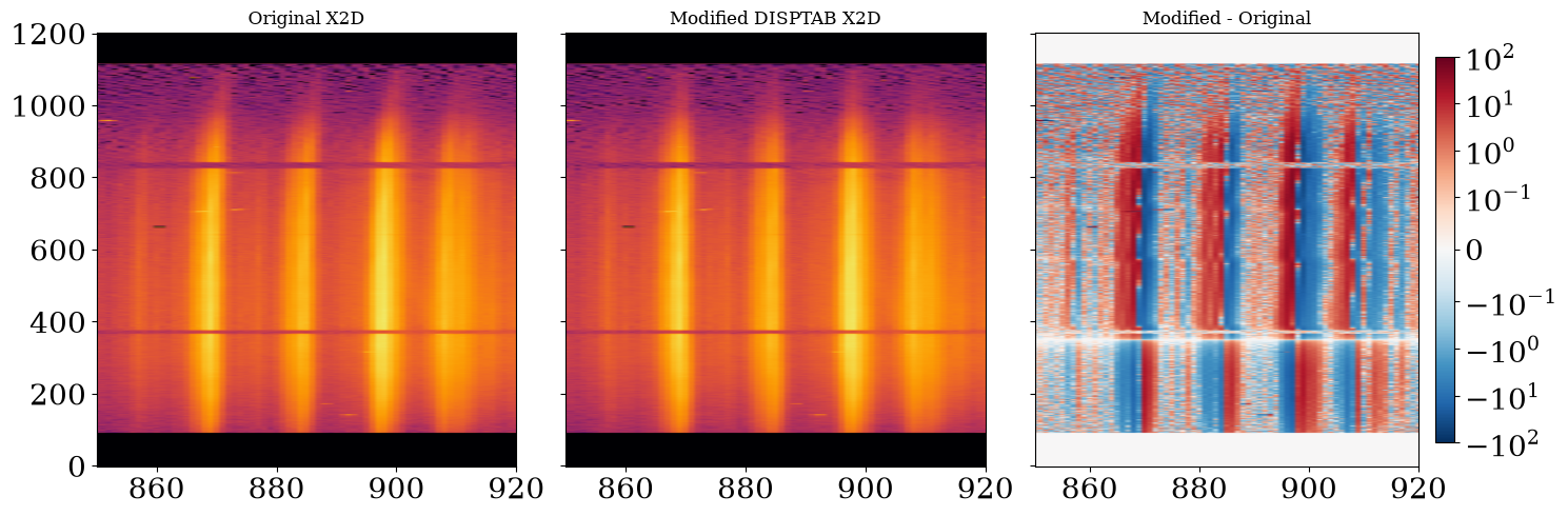
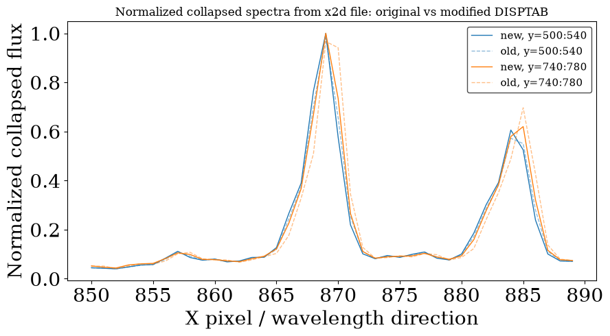
In the plot here below you can select the xrange equal to the range were you see clear emission lines in the 2D plot above.

xrange = slice(850, 890)

yranges = [
    slice(500, 540),
    slice(740, 780),
]

x = np.arange(x2d.shape[1])[xrange]

fig, ax = plt.subplots(figsize=(9, 5))

for yrange in yranges:
    prof_new = np.nansum(x2d[yrange, xrange], axis=0)
    prof_old = np.nansum(x2d_orig[yrange, xrange], axis=0)

    norm = np.nanmax(prof_new)

    prof_new_norm = prof_new / norm
    prof_old_norm = prof_old / norm

    line, = ax.plot(
        x,
        prof_new_norm,
        label=f'new, y={yrange.start}:{yrange.stop}'
    )

    ax.plot(
        x,
        prof_old_norm,
        linestyle='--',
        color=line.get_color(),
        alpha=0.5,
        label=f'old, y={yrange.start}:{yrange.stop}'
    )

ax.set_xlabel('X pixel / wavelength direction')
ax.set_ylabel('Normalized collapsed flux')
ax.set_title('Normalized collapsed spectra from x2d file: original vs modified DISPTAB')
ax.legend(fontsize=11)
fig.tight_layout()
plt.savefig(mypath / f'normalized_collapsed_spectra_original_vs_modified_DISPTAB_{grating}_{cenwave}_{lamp}.png', dpi=300)
plt.show()

Conclusions

Updating the DISPTAB reference file in this way allows the wavelength correction to be incorporated directly into the calibration reference file, enabling the generation of corrected x2d products and the extraction of 1D spectra with stistools.x1d without specifying an xoffset. However, the resulting DISPTAB is specific to the particular grating setting and observation analyzed and should not be used for other datasets.

About this Notebook

Author: Matilde Mingozzi

Updated On: 2026-07-10

This tutorial was generated to be in compliance with the STScI style guides and would like to cite the Jupyter guide in particular.

Citations

If you use astropy, matplotlib, astroquery, scipy, or numpy for published research, please cite the authors. Follow these links for more information about citations:

• Citing scipy

• Citing matplotlib

• Citing numpy

• Citing astroquery

• Citing astropy

---

Top of Page