WFC3/UVIS: Equalizing Amplifier Offsets in FLC/FLT Images

---

Learning Goals

In this tutorial you will:

• Download data from MAST

• Build a segmentation map

• Measure the background in each quadrant

• Apply flat-field corrections and equalize amp bias levels

Table of Contents

1. Introduction

2. Setup

3. Imports

4. Inputs

5. Step 1: Build Source Segmentation Maps

6. Step 2: Measure Median Background Per Amp

7. Step 3: Compute Per-Amp Offsets

8. Step 4: Apply the Flat-Field Correction and Equalize Amps

9. Step 5: Inspect the Results

10. Step 6: Re-Drizzle the Corrected Images

11. Summary

1. Introduction

In this tutorial, you will be guided through how to determine the amplifier-dependent bias offsets in a Wide Field Camera 3 (WFC3) UVIS channel image and equalize the bias levels in each amplifier (amp) to the average across the image.

The amp-offset correction workflow in this notebook follows the method from Sunnquist (2019) and uses much of the same code. An overview of the steps we will take to achieve this is as follows:

1. Build a source segmentation map to mask stars and galaxies before measuring sky backgrounds

2. Measure the background level in each amp quadrant (avoiding sources) and the mean over all amps

3. Compute per-amp offsets relative to the overall mean background

4. Multiply these offsets by the flat field to account for sensitivity variations.

5. Subtract the resulting amp-by-amp corrections from the original FLC/FLT data.

If necessary, users should then re-drizzle their data using the corrected images to create new DRZ/DRC files after completing the above steps.

The WFC3/UVIS detector has four amplifiers (A, B, C, D), each covering one quadrant of the 4Kx4K pixel field. Even after the standard calwf3 pipeline reduction, small offsets to the bias level can persist between quadrants. These offsets are relatively constant across each quadrant, and sometimes show up as visible to the eye, with some amps brighter than others.

WFC3/UVIS Amplifier Layout

The UVIS detector spans two CCDs (chips), each with two amps. The science data live in FITS extensions 1 (chip 2, lower) and 4 (chip 1, upper).

┌──────────────────────┐
│   Amp A  │  Amp B    │  ← Extension 4, UVIS1
├──────────────────────┤
│   Amp C  │  Amp D    │  ← Extension 1, UVIS2
└──────────────────────┘

Within each extension, the left half corresponds to one amp and the right half to the other.

2. Setup

Environment

This notebook requires a working STScI Conda environment, stenv. If you do not have one, follow the stenv installation guide before proceeding.

This notebook requires users to install the packages listed in the requirements.txt file located in the notebook’s sub-folder on the GitHub repository. Most of these packages should already exist in your stenv environment, but if you happen to be missing any required packages, they can be installed from the requirements.txt file with pip install.

3. Imports

For this notebook we import:

Package	Purpose
glob	File handling
matplotlib.pyplot	Displaying images and visualizing offsets
numpy	Handling arrays
os	System commands
shutil	File and directory clean up
astropy.io.fits	Reading and modifying FITS files
astropy.convolution	Tools to smooth the background of images
astropy.stats	Tools to smooth the background of images
astroquery.mast.Observations	Downloading FLC and DRC data from MAST
photutils.segmentation	Creating source masks
drizzlepac	Aligning and re-combining images

import glob
import os
import shutil

import numpy as np
import matplotlib.pyplot as plt
%matplotlib inline

from astropy.io import fits
from astropy.convolution import convolve, Gaussian2DKernel
from astropy.stats import gaussian_fwhm_to_sigma
from astroquery.mast import Observations
from photutils.segmentation import detect_sources, detect_threshold
from drizzlepac import tweakreg, astrodrizzle
from drizzlepac.processInput import getMdriztabPars

4. Inputs

Downloading an Example Image

For the purposes of this tutorial, we will download a set of WFC3/UVIS images with clear amp-dependent offsets and work through the steps to correct the offsets. Alternatively, you could download your own data to run through this pipeline! We recommend working through the example data first.

We will use Astroquery to retrieve files. We query for data from the Mikulski Archive for Space Telescopes (MAST) as follows:

# Define the dataset you want. In this case, we are using the obsID for the set of two example exposures
obsID = 'ifcpc6030'
# Query observations by obs_id
obs_table = Observations.query_criteria(obs_id=obsID)

# Get list of data products
data_products = Observations.get_product_list(obs_table)
data_products

Table masked=True length=50

obsID	obs_collection	dataproduct_type	obs_id	description	type	dataURI	productType	productGroupDescription	productSubGroupDescription	productDocumentationURL	project	prvversion	proposal_id	productFilename	size	parent_obsid	dataRights	calib_level	filters
str9	str3	str5	str37	str64	str1	str69	str9	str28	str11	str1	str7	str19	str5	str52	int64	str9	str6	int64	str9
381172864	HST	image	ifcpc6030	DADS JIF file	D	mast:HST/product/ifcpc6030_jif.fits	AUXILIARY	--	JIF	--	CALWF3	--	17833	ifcpc6030_jif.fits	60480	381172864	PUBLIC	1	F336W
381172864	HST	image	ifcpc6030	DADS JIT file	D	mast:HST/product/ifcpc6030_jit.fits	AUXILIARY	--	JIT	--	CALWF3	--	17833	ifcpc6030_jit.fits	57600	381172864	PUBLIC	1	F336W
381172864	HST	image	ifcpc6030	DADS SPT file - Engineering telemetry ACS/WFC3/NICMOS/COS/STIS	D	mast:HST/product/ifcpc6030_spt.fits	AUXILIARY	--	SPT	--	CALWF3	--	17833	ifcpc6030_spt.fits	178560	381172864	PUBLIC	1	F336W
381172864	HST	image	ifcpc6030	Pipeline processing logs	D	mast:HST/product/ifcpc6030_trl.fits	AUXILIARY	--	TRL	--	CALWF3	--	17833	ifcpc6030_trl.fits	478080	381172864	PUBLIC	1	F336W
381172864	HST	image	ifcpc6030	DADS ASN file - Association ACS/WFC3/STIS	D	mast:HST/product/ifcpc6030_asn.fits	AUXILIARY	Minimum Recommended Products	ASN	--	CALWF3	3.7.3 (Jan-07-2026)	17833	ifcpc6030_asn.fits	11520	381172864	PUBLIC	3	F336W
381172864	HST	image	ifcpc6030	DADS LOG file	D	mast:HST/product/ifcpc6030_log.txt	INFO	--	LOG	--	CALWF3	--	17833	ifcpc6030_log.txt	146130	381172864	PUBLIC	1	F336W
381172864	HST	image	ifcpc6030	Preview-Full	D	mast:HST/product/ifcpc6030_drc.jpg	PREVIEW	--	--	--	CALWF3	3.7.3 (Jan-07-2026)	17833	ifcpc6030_drc.jpg	3733405	381172864	PUBLIC	3	F336W
381172864	HST	image	ifcpc6030	Preview-Full	D	mast:HST/product/ifcpc6030_drz.jpg	PREVIEW	--	--	--	CALWF3	3.7.3 (Jan-07-2026)	17833	ifcpc6030_drz.jpg	4074142	381172864	PUBLIC	3	F336W
381172864	HST	image	ifcpc6030	DADS DRC file - CTE-corrected calibrated combined image ACS/WFC3	D	mast:HST/product/ifcpc6030_drc.fits	SCIENCE	Minimum Recommended Products	DRC	--	CALWF3	3.7.3 (Jan-07-2026)	17833	ifcpc6030_drc.fits	223217280	381172864	PUBLIC	3	F336W
...	...	...	...	...	...	...	...	...	...	...	...	...	...	...	...	...	...	...	...
381174603	HST	image	hst_17833_c6_wfc3_uvis_f336w_ifcpc6	HAP trailer file	D	mast:HST/product/hst_17833_c6_wfc3_uvis_f336w_ifcpc6_trl.txt	AUXILIARY	--	TRL	--	HAP-SVM	DrizzlePac 3.10.0	17833	hst_17833_c6_wfc3_uvis_f336w_ifcpc6_trl.txt	16937	381172864	PUBLIC	3	F336W
381174603	HST	image	hst_17833_c6_wfc3_uvis_f336w_ifcpc6	Preview-Full	D	mast:HST/product/hst_17833_c6_wfc3_uvis_f336w_ifcpc6_drc.jpg	PREVIEW	--	--	--	HAP-SVM	DrizzlePac 3.10.0	17833	hst_17833_c6_wfc3_uvis_f336w_ifcpc6_drc.jpg	4229051	381172864	PUBLIC	3	F336W
381174603	HST	image	hst_17833_c6_wfc3_uvis_f336w_ifcpc6	HAP fits science image	D	mast:HST/product/hst_17833_c6_wfc3_uvis_f336w_ifcpc6_drc.fits	SCIENCE	--	DRC	--	HAP-SVM	DrizzlePac 3.10.0	17833	hst_17833_c6_wfc3_uvis_f336w_ifcpc6_drc.fits	443459520	381172864	PUBLIC	3	F336W
381174603	HST	image	hst_17833_c6_wfc3_uvis_f336w_ifcpc6	HAP source catalog	D	mast:HST/product/hst_17833_c6_wfc3_uvis_f336w_ifcpc6_point-cat.ecsv	SCIENCE	--	POINT-CAT	--	HAP-SVM	DrizzlePac 3.10.0	17833	hst_17833_c6_wfc3_uvis_f336w_ifcpc6_point-cat.ecsv	1171901	381172864	PUBLIC	3	F336W
381174603	HST	image	hst_17833_c6_wfc3_uvis_f336w_ifcpc6	HAP source catalog	D	mast:HST/product/hst_17833_c6_wfc3_uvis_f336w_ifcpc6_segment-cat.ecsv	SCIENCE	--	SEGMENT-CAT	--	HAP-SVM	DrizzlePac 3.10.0	17833	hst_17833_c6_wfc3_uvis_f336w_ifcpc6_segment-cat.ecsv	4281757	381172864	PUBLIC	3	F336W
381174609	HST	image	hst_17833_c6_wfc3_uvis_total_ifcpc6	HAP trailer file	D	mast:HST/product/hst_17833_c6_wfc3_uvis_total_ifcpc6_trl.txt	AUXILIARY	--	TRL	--	HAP-SVM	DrizzlePac 3.11.0	17833	hst_17833_c6_wfc3_uvis_total_ifcpc6_trl.txt	261468	381172864	PUBLIC	3	detection
381174609	HST	image	hst_17833_c6_wfc3_uvis_total_ifcpc6	Preview-Full	D	mast:HST/product/hst_17833_c6_wfc3_uvis_total_ifcpc6_drc.jpg	PREVIEW	--	--	--	HAP-SVM	DrizzlePac 3.11.0	17833	hst_17833_c6_wfc3_uvis_total_ifcpc6_drc.jpg	5049606	381172864	PUBLIC	3	detection
381174609	HST	image	hst_17833_c6_wfc3_uvis_total_ifcpc6	HAP fits science image	D	mast:HST/product/hst_17833_c6_wfc3_uvis_total_ifcpc6_drc.fits	SCIENCE	--	DRC	--	HAP-SVM	DrizzlePac 3.11.0	17833	hst_17833_c6_wfc3_uvis_total_ifcpc6_drc.fits	443473920	381172864	PUBLIC	3	detection
381174609	HST	image	hst_17833_c6_wfc3_uvis_total_ifcpc6	HAP source catalog	D	mast:HST/product/hst_17833_c6_wfc3_uvis_total_ifcpc6_point-cat.ecsv	SCIENCE	--	POINT-CAT	--	HAP-SVM	DrizzlePac 3.11.0	17833	hst_17833_c6_wfc3_uvis_total_ifcpc6_point-cat.ecsv	198643	381172864	PUBLIC	3	detection
381174609	HST	image	hst_17833_c6_wfc3_uvis_total_ifcpc6	HAP source catalog	D	mast:HST/product/hst_17833_c6_wfc3_uvis_total_ifcpc6_segment-cat.ecsv	SCIENCE	--	SEGMENT-CAT	--	HAP-SVM	DrizzlePac 3.11.0	17833	hst_17833_c6_wfc3_uvis_total_ifcpc6_segment-cat.ecsv	308681	381172864	PUBLIC	3	detection

# Filter for calibrated science products (in this case, FLC and DRC files from CALWF3)
filtered_products = Observations.filter_products(
    data_products,
    productSubGroupDescription=["FLC", "DRC",],
    project='CALWF3' 
)

filtered_products

Table masked=True length=3

obsID	obs_collection	dataproduct_type	obs_id	description	type	dataURI	productType	productGroupDescription	productSubGroupDescription	productDocumentationURL	project	prvversion	proposal_id	productFilename	size	parent_obsid	dataRights	calib_level	filters
str9	str3	str5	str37	str64	str1	str69	str9	str28	str11	str1	str7	str19	str5	str52	int64	str9	str6	int64	str9
381172864	HST	image	ifcpc6030	DADS DRC file - CTE-corrected calibrated combined image ACS/WFC3	D	mast:HST/product/ifcpc6030_drc.fits	SCIENCE	Minimum Recommended Products	DRC	--	CALWF3	3.7.3 (Jan-07-2026)	17833	ifcpc6030_drc.fits	223217280	381172864	PUBLIC	3	F336W
381172866	HST	image	ifcpc6wdq	DADS FLC file - CTE-corrected calibrated exposure ACS/WFC3	S	mast:HST/product/ifcpc6wdq_flc.fits	SCIENCE	--	FLC	--	CALWF3	3.7.3 (Jan-07-2026)	17833	ifcpc6wdq_flc.fits	168675840	381172864	PUBLIC	2	F336W
381172869	HST	image	ifcpc6wfq	DADS FLC file - CTE-corrected calibrated exposure ACS/WFC3	S	mast:HST/product/ifcpc6wfq_flc.fits	SCIENCE	--	FLC	--	CALWF3	3.7.3 (Jan-07-2026)	17833	ifcpc6wfq_flc.fits	168675840	381172864	PUBLIC	2	F336W

# Download
manifest = Observations.download_products(
    filtered_products,
    mrp_only=False,    
    download_dir="./"  # setting the download path to the current working directory
)

print(manifest)

INFO: Found cached file ./mastDownload/HST/ifcpc6030/ifcpc6030_drc.fits with expected size 223217280. [astroquery.query]

Downloading URL https://mast.stsci.edu/api/v0.1/Download/file?uri=mast:HST/product/ifcpc6wdq_flc.fits to ./mastDownload/HST/ifcpc6wdq/ifcpc6wdq_flc.fits ...

 [Done]

Downloading URL https://mast.stsci.edu/api/v0.1/Download/file?uri=mast:HST/product/ifcpc6wfq_flc.fits to ./mastDownload/HST/ifcpc6wfq/ifcpc6wfq_flc.fits ...

 [Done]

                   Local Path                    Status  Message URL 
----------------------------------------------- -------- ------- ----
./mastDownload/HST/ifcpc6030/ifcpc6030_drc.fits COMPLETE    None None
./mastDownload/HST/ifcpc6wdq/ifcpc6wdq_flc.fits COMPLETE    None None
./mastDownload/HST/ifcpc6wfq/ifcpc6wfq_flc.fits COMPLETE    None None

Please note: If you are working on a set of images, it is important to place all FLC (or FLT) files for a single filter in a working directory and set the path. Code is provided below to do this. All files must use the same filter because the flat-field correction step relies on the PFLTFILE keyword in the primary header, which is filter-dependent.

# Directory where files were downloaded
download_dir = "mastDownload"

# Loop over all FITS files
for root, dirs, files in os.walk(download_dir):
    for file in files:
        if file.endswith("flc.fits"):
            filepath = os.path.join(root, file)

            try:
                # Read FITS header
                with fits.open(filepath) as hdul:
                    hdr = hdul[0].header

                # Get filter name
                filt = hdr.get("FILTER", None)

                if filt is None or filt == "":
                    print(f"Skipping {file}: no filter found")
                    continue

                # Create destination directory (one level below cwd)
                dest_dir = os.path.join(os.getcwd(), filt)
                os.makedirs(dest_dir, exist_ok=True)

                # Move file
                dest_path = os.path.join(dest_dir, file)
                shutil.move(filepath, dest_path)

                print(f"Moved {file} → {dest_dir}")

            except Exception as e:
                print(f"Error processing {file}: {e}")

Moved ifcpc6wdq_flc.fits → /home/runner/work/hst_notebooks/hst_notebooks/notebooks/WFC3/uvis_amp_equalization/F336W

Moved ifcpc6wfq_flc.fits → /home/runner/work/hst_notebooks/hst_notebooks/notebooks/WFC3/uvis_amp_equalization/F336W

# Filter-specific directory containing the FLC/FLT files (in this case, the exposures we care about are in './F336M/')
filter_dir = './F336W'

os.chdir(filter_dir)
# Glob to select your science files
files = sorted(glob.glob('*flc.fits'))

print(f'Found {len(files)} input file(s):')
for f in files:
    print(f'  {f}')

Found 2 input file(s):
  ifcpc6wdq_flc.fits
  ifcpc6wfq_flc.fits

Let’s take a look at our images. Below, we plot the science data of our two example images. Using a narrow stretch, we can see the amp-to-amp background offsets by eye, with some quadrants appearing darker/lighter than others.

for fname in files:

    # Load both chips
    chip2 = fits.getdata(fname, ext=1)  # UVIS2
    chip1 = fits.getdata(fname, ext=4)  # UVIS1

    # Stack vertically 
    full = np.vstack([chip2, chip1])

    # Tight stretch to highlight amp offsets
    vmin, vmax = np.percentile(full, [45, 55])

    plt.figure(figsize=(8, 10))
    plt.imshow(full, origin='lower', cmap='gray', vmin=vmin, vmax=vmax)
    plt.colorbar(label="Electrons ($e^{-}$)", shrink=0.6,)
    plt.title(fname)
    plt.xlabel("X")
    plt.ylabel("Y")
    plt.show()

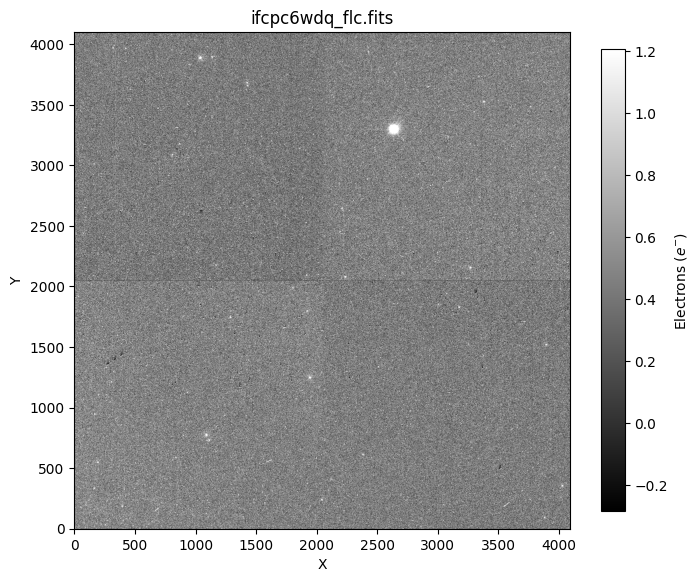
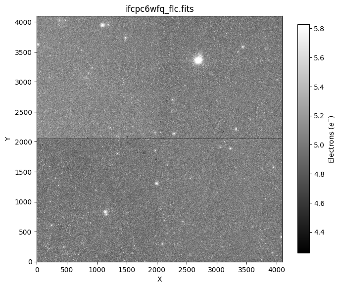
Lastly, we need to set our iref path to point to a directory containing WFC3 reference files. We will use the Calibration Reference Data System (CRDS), which automatically downloads the right reference files on demand.

crds_path = os.path.expanduser("~") + "/crds_cache"
os.environ["CRDS_PATH"] = crds_path
os.environ["CRDS_SERVER_URL"] = "https://hst-crds.stsci.edu"
os.environ["iref"] = os.path.join(crds_path, "references/hst/wfc3/")

5. Step 1 — Build Source Segmentation Maps

Before we can measure the background sky level in each amp quadrant, we need to identify and mask any pixels that belong to real sources (stars, galaxies, etc.). We do this using a segmentation map, in which pixels belonging to a detected source are labeled with a nonzero integer, and pure-sky pixels are labeled 0.

We use the photutils package to detect sources and mask them for our image. We mask only sources that span 3 or more pixels and are at least 1 standard deviation per pixel above the background. A 3 sigma Gaussian smoothing kernel is applied before source detection to average out single bright pixels from non-source artifacts such as hot pixels or cosmic rays. We use a low signal-to-noise-ratio (SNR) threshold of 1 standard deviation because we would rather over-mask a few sky pixels than accidentally include a faint source wing in our background estimate, which would bias the amp-level measurements.

The segmentation maps (“segmaps”) are written out as {filename}_seg_ext_{1|4}.fits so they can be reused in later steps without repeating the detection.

def make_segmap(f, smoothing_sigma=3, threshold_sigma=1.0, source_pixel_span=3, overwrite=True):
    """
    Build a source segmentation map for each science extension of a UVIS file.

    Parameters
    ----------
    f : str
        Path to the FLC/FLT FITS file.
    smoothing_sigma : float, optional
        FWHM in pixels of the Gaussian smoothing kernel applied before source
        detection to average out single-pixel artifacts such as hot pixels or
        cosmic rays. Default is 3.
    threshold_sigma : float, optional
        The sigma (signal-to-noise) threshold above which a pixel is considered
        part of a source. Default is 1.0.
    source_pixel_span : int, optional
        Minimum number of contiguous pixels required for a detection to be
        considered a source. Default is 3.
    overwrite : bool, optional
        If True, regenerate the segmap even if it already exists on disk.
        Default is True.

    Outputs
    -------
    {f}_seg_ext_1.fits, {f}_seg_ext_4.fits
        Segmentation maps for each SCI extension of the FITS file.
    """
    sigma = smoothing_sigma * gaussian_fwhm_to_sigma  
    kernel = Gaussian2DKernel(sigma, x_size=3, y_size=3)
    kernel.normalize()

    for ext in [1, 4]:
        outfile = f.replace('.fits', f'_seg_ext_{ext}.fits')
        if os.path.exists(outfile) and not overwrite:
            print(f'  Segmap already exists, skipping: {outfile}')
            continue

        data = fits.getdata(f, ext)
        threshold = detect_threshold(data, nsigma=threshold_sigma)
        convolved_data = convolve(data, kernel, normalize_kernel=True)
        segm = detect_sources(convolved_data, threshold, npixels=source_pixel_span)

        fits.writeto(outfile, segm.data.astype(np.int32), overwrite=True)
        print(f'  Written: {outfile}')

print('Building segmentation maps...\n')
for f in files:
    print(f'Processing {f}')
    make_segmap(f, overwrite=False)
print('\nDone.')

Building segmentation maps...

Processing ifcpc6wdq_flc.fits
  Segmap already exists, skipping: ifcpc6wdq_flc_seg_ext_1.fits
  Segmap already exists, skipping: ifcpc6wdq_flc_seg_ext_4.fits
Processing ifcpc6wfq_flc.fits
  Segmap already exists, skipping: ifcpc6wfq_flc_seg_ext_1.fits
  Segmap already exists, skipping: ifcpc6wfq_flc_seg_ext_4.fits

Done.

Inspect the segmentation maps

We want to visually verify that the segmaps capture the sources without over-masking too much sky. In the plot below, we show our original science data on the left, and the segmentation map on the right with masked (source) pixels shown in yellow and sky pixels in dark purple/blue. In our example images, the brightest source falls on the upper chip (UVIS1, SCI extension 4).

for fname in files:
    fname
    # Load both chips
    data_ext1 = fits.getdata(fname, 1)  # UVIS2
    data_ext4 = fits.getdata(fname, 4)  # UVIS1

    segmap_ext1 = fits.getdata(fname.replace('.fits', '_seg_ext_1.fits'))
    segmap_ext4 = fits.getdata(fname.replace('.fits', '_seg_ext_4.fits'))

    # Stack vertically
    data_full = np.vstack([data_ext1, data_ext4])
    segmap_full = np.vstack([segmap_ext1, segmap_ext4])

    vmin, vmax = np.percentile(data_full, [45, 55])

    fig, axes = plt.subplots(1, 2, figsize=(14, 8))

    axes[0].imshow(data_full, origin='lower', cmap='gray', vmin=vmin, vmax=vmax)
    axes[0].set_title('Science image (both chips)', fontsize=13)
    axes[0].set_xlabel('X pixel')
    axes[0].set_ylabel('Y pixel')

    axes[1].imshow(segmap_full > 0, origin='lower', cmap='viridis')
    axes[1].set_title('Source mask (yellow = masked)', fontsize=13)
    axes[1].set_xlabel('X pixel')

    plt.suptitle(os.path.basename(fname), fontsize=12)
    plt.tight_layout()
    plt.show()

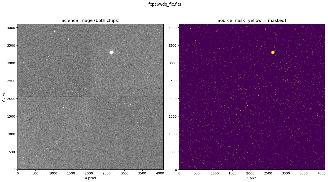
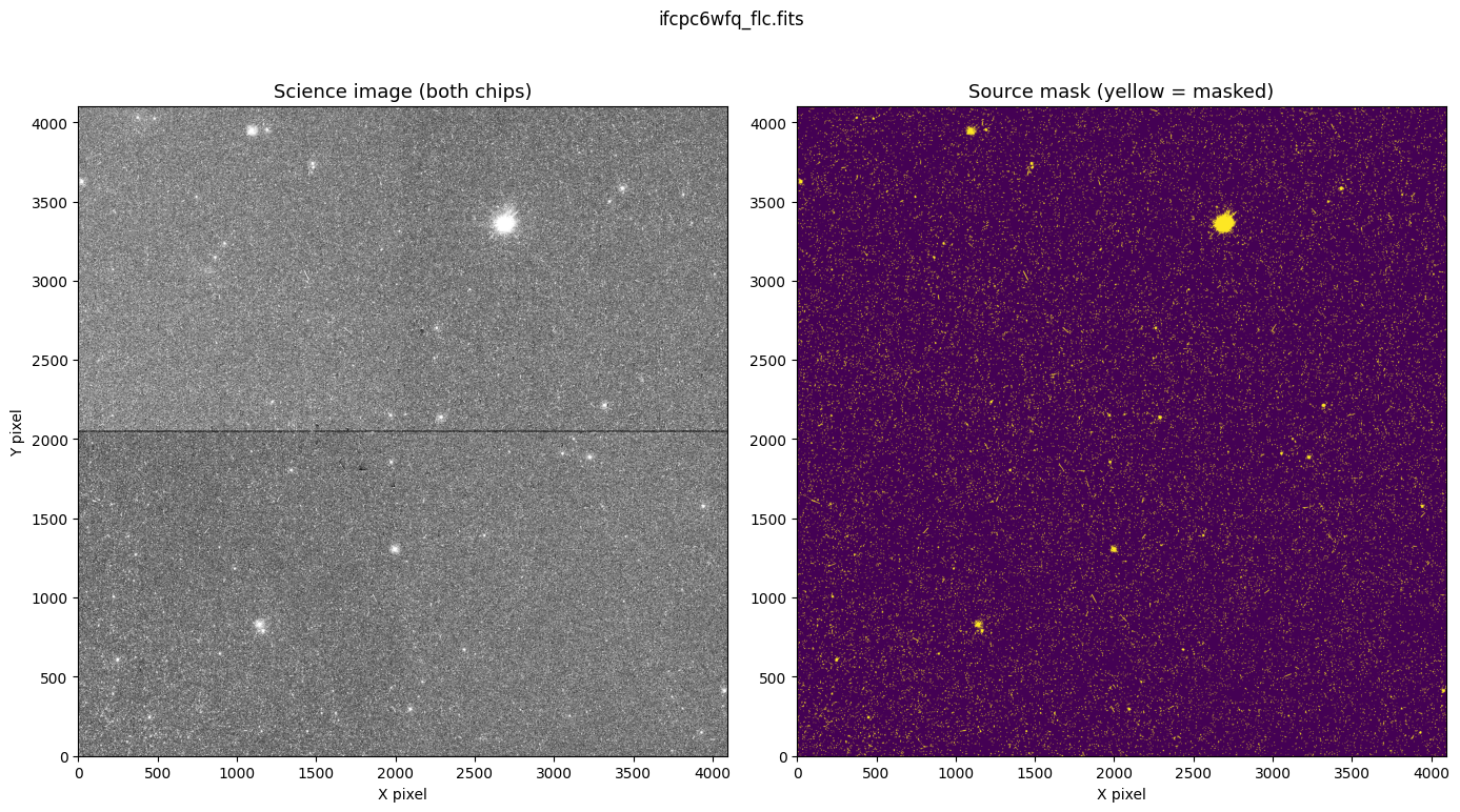
6. Step 2 — Measure Median Background Per Amp

With sources masked, we can now measure a robust background level for each of the four amp quadrants. We use the median rather than the mean because it is less sensitive to residual contamination from faint sources or bad pixels.

Each UVIS science extension covers two amps. We split each extension exactly in half along the column axis to grab each amp individually.

Source pixels (segmap > 0) are set to NaN before the split so that np.nanmedian automatically ignores them.

def measure_amp_levels(f):
    """
    Measure the median sky background in each of the four UVIS amp quadrants.

    Parameters
    ----------
    f : str
        Path to the FLC/FLT FITS file.

    Returns
    -------
    amp_levels : list of float
        [median_C, median_D, median_A, median_B]  (electrons)
    amp_average : float
        Mean of all four amp medians.
    """
    amp_levels = []

    for ext in [1, 4]:
        data = fits.getdata(f, ext).astype(float)
        segmap = fits.getdata(f.replace('.fits', f'_seg_ext_{ext}.fits'))

        # Mask sources
        data[segmap > 0] = np.nan

        # Split into left (amp A/C) and right (amp B/D) halves
        left, right = np.split(data, 2, axis=1)

        amp_levels.append(np.nanmedian(left))
        amp_levels.append(np.nanmedian(right))

    amp_average = np.nanmean(amp_levels)
    return amp_levels, amp_average

print(f'{"File":<35}  {"Amp A":>8}  {"Amp B":>8}  {"Amp C":>8}  {"Amp D":>8}  {"Mean":>8}')
print('-' * 85)

all_levels = {}
for f in files: # in our example case we only have two files
    levels, avg = measure_amp_levels(f)
    all_levels[f] = (levels, avg)
    C, D, A, B = levels  # extension 1 (UVIS2, amps C & D) are appended to the list first
    print(f'{os.path.basename(f):<35}  {A:8.4f}  {B:8.4f}  {C:8.4f}  {D:8.4f}  {avg:8.4f}')

File                                    Amp A     Amp B     Amp C     Amp D      Mean
-------------------------------------------------------------------------------------

ifcpc6wdq_flc.fits                     0.1432    0.5373    0.6042    0.2598    0.3861

ifcpc6wfq_flc.fits                     5.2840    4.7085    4.3501    4.6941    4.7592

7. Step 3 — Compute the Per-Amp Offsets

The offset for each amplifier quadrant is the deviation of its median background from the overall mean (the mean of the per-amp medians).

A positive offset means that the amp reads slightly high relative to the average, and we will want to subtract the offset to correct for it. After the correction, the four quadrant levels should all be approximately equal to the overall mean across all four amps.

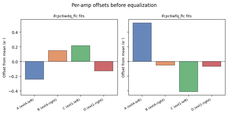
Below, we plot the per-amp offsets from the mean before equalization as a bar chart for each image and explicitly print the offset information.

# Visualise the offsets for each file as a bar chart
print('Per-amp offsets from mean before equalization (e-)')
print(f'{"File":<30} {"A":>8}  {"B":>8}  {"C":>8}  {"D":>8}')
print('-' * 85)

amp_labels = ['A (ext4-left)', 'B (ext4-right)', 'C (ext1-left)', 'D (ext1-right)']
colors = ['#4C72B0', '#DD8452', '#55A868', '#C44E52']

# fig, axes = plt.subplots(1, len(files), figsize=(4 * len(files), 4), sharey=True)
# if len(files) == 1:
#     axes = [axes]

for ax, f in zip(axes, files):
    levels, avg = all_levels[f]
    offsets = [lv - avg for lv in levels]
    reordered = [offsets[i] for i in [2, 3, 0, 1]] 
    print(f'{os.path.basename(fname):<30}  {reordered[0]:8.4f}  {reordered[1]:8.4f} {reordered[2]:8.4f}  {reordered[3]:8.4f}')
    bars = ax.bar(amp_labels, reordered, color=colors, alpha=0.85, edgecolor='black', linewidth=0.6)
    ax.axhline(0, color='black', linewidth=0.8, linestyle='--')
    ax.set_title(os.path.basename(f), fontsize=9)
    ax.set_xticklabels(amp_labels, rotation=30, ha='right', fontsize=8)
    ax.set_ylabel('Offset from mean (e⁻)', fontsize=9)

fig.suptitle('Per-amp offsets before equalization', fontsize=12, y=0.98)
plt.tight_layout()
plt.show()

Per-amp offsets from mean before equalization (e-)
File                                  A         B         C         D
-------------------------------------------------------------------------------------
ifcpc6wfq_flc.fits               -0.2429    0.1512   0.2181   -0.1263
ifcpc6wfq_flc.fits                0.5248   -0.0507  -0.4091   -0.0651

<Figure size 640x480 with 0 Axes>

8. Step 4 — Apply the Flat-Field Correction and Equalize Amps

The FLC/FLT data have already been “flat-fielded” (divided by the flat-field image). The residual amp offsets, therefore, have also been modulated by the flat. To correct for this, we multiply the amp-to-amp scalar offset arrays by the flat before subtracting from the science data. This ensures the subtracted correction has exactly the same pixel-level shape as the bias offset would have had before flat-fielding, producing a cleaner result.

The flat-field file is identified from the PFLTFILE keyword in the primary header and loaded from the $iref reference file directory.

def equalize_amps(f, multiply_flat=True, overwrite=True):
    """
    Equalize the four UVIS amp levels in an FLC/FLT image.

    For each amp quadrant the median background (computed with sources masked)
    is compared to the mean of all four quadrants.  The difference
    (optionally multiplied by the flat field) is subtracted from the
    original science data.

    Parameters
    ----------
    f : str
        Path to the FLC/FLT FITS file.  Segmaps must already exist (Step 1).
    multiply_flat : bool
        If True (recommended), scale the offset by the flat field before
        subtracting so that the correction accounts for sensitivity variations
        across each quadrant. (Default: True)
    overwrite: bool
        Overwrite existing output file with the same name, if True. (Default: False)

    Outputs
    -------
    {f}_eq.fits
        A copy of the input file with equalized amp levels written to SCI
        extensions 1 and 4.
    """
    outfile = f.replace('.fits', '_eq.fits')
    if not overwrite and os.path.isfile(outfile):
        print(f'  Output already exists, skipping: {outfile}')
        return outfile

    h = fits.open(f)

    # Locate the flat-field reference file if needed
    if multiply_flat:
        pflt_key = h[0].header['PFLTFILE'].replace('iref$', '')
        iref = os.environ['iref']
        os.system(f'crds sync --hst --files {pflt_key} --output-dir {iref}')
        flat_file = os.path.join(os.environ['iref'], pflt_key)
        print(f'  Using flat field: {os.path.basename(flat_file)}')

    #  Collect the median background level in each of the 4 amp quadrants 
    amp_levels = []
    for ext in [1, 4]:
        data = h[ext].data.astype(float).copy()
        segmap = fits.getdata(f.replace('.fits', f'_seg_ext_{ext}.fits'))
        data[segmap > 0] = np.nan          # mask sources
        left, right = np.split(data, 2, axis=1)
        amp_levels.append(np.nanmedian(left))
        amp_levels.append(np.nanmedian(right))

    amp_average = np.nanmean(amp_levels)

    print(f'  Amp medians  : A={amp_levels[2]:.4f}  B={amp_levels[3]:.4f}  '
          f'C={amp_levels[0]:.4f}  D={amp_levels[1]:.4f}')
    print(f'  Overall mean   : {amp_average:.4f}')
    offsets = [lv - amp_average for lv in amp_levels]
    print(f'  Offsets (C,D,A,B): {[f"{o:.4f}" for o in offsets]}')

    # Subtract the offset from the original data 

    for ext in [1, 4]:
        data_orig = h[ext].data.astype(float).copy()
        left_orig, right_orig = np.split(data_orig, 2, axis=1)

        # Source-masked copy for measuring 
        data_masked = data_orig.copy()
        segmap = fits.getdata(f.replace('.fits', f'_seg_ext_{ext}.fits'))
        data_masked[segmap > 0] = np.nan
        left_m, right_m = np.split(data_masked, 2, axis=1)

        if multiply_flat:
            flat = fits.getdata(flat_file, ext).astype(float)
            flat_left, flat_right = np.split(flat, 2, axis=1)
            correction_left = (np.nanmedian(left_m) - amp_average) * flat_left
            correction_right = (np.nanmedian(right_m) - amp_average) * flat_right
        else:
            correction_left = np.nanmedian(left_m) - amp_average
            correction_right = np.nanmedian(right_m) - amp_average

        left_new = left_orig - correction_left
        right_new = right_orig - correction_right

        h[ext].data = np.concatenate([left_new, right_new], axis=1).astype('float32')

    h.writeto(outfile, overwrite=True)
    h.close()
    print(f'  Written: {outfile}')
    return outfile

print('Equalizing amp levels...\n')
eq_files = []
for f in files:
    print(f'Processing {f}')
    outfile = equalize_amps(f, multiply_flat=True)
    eq_files.append(outfile)
    print()
print('Done.')

Equalizing amp levels...

Processing ifcpc6wdq_flc.fits

CRDS - INFO -  Symbolic context 'hst-latest' resolves to 'hst_1345.pmap'
CRDS - INFO -  Reorganizing 0 references from 'instrument' to 'flat'
CRDS - INFO -  Reorganizing from 'instrument' to 'flat' cache,  removing instrument directories.
CRDS - INFO -  Syncing explicitly listed files.
CRDS - INFO -  0 errors
CRDS - INFO -  0 warnings
CRDS - INFO -  4 infos

  Using flat field: zcv2053ki_pfl.fits

  Amp medians  : A=0.1432  B=0.5373  C=0.6042  D=0.2598
  Overall mean   : 0.3861
  Offsets (C,D,A,B): ['0.2181', '-0.1263', '-0.2429', '0.1512']

  Written: ifcpc6wdq_flc_eq.fits

Processing ifcpc6wfq_flc.fits

CRDS - INFO -  Symbolic context 'hst-latest' resolves to 'hst_1345.pmap'
CRDS - INFO -  Reorganizing 0 references from 'instrument' to 'flat'
CRDS - INFO -  Reorganizing from 'instrument' to 'flat' cache,  removing instrument directories.
CRDS - INFO -  Syncing explicitly listed files.
CRDS - INFO -  0 errors
CRDS - INFO -  0 warnings
CRDS - INFO -  4 infos

  Using flat field: zcv2053ki_pfl.fits

  Amp medians  : A=5.2840  B=4.7085  C=4.3501  D=4.6941
  Overall mean   : 4.7592
  Offsets (C,D,A,B): ['-0.4091', '-0.0651', '0.5248', '-0.0507']

  Written: ifcpc6wfq_flc_eq.fits

Done.

9. Step 5 — Inspect the Results

We now compare the per-amp medians before and after equalization to verify that the correction worked as expected. After equalization all four quadrant medians should be within a small fraction of an electron of each other.

print('Amp medians before and after equalization\n')
print(f'{"File":<30}  {"State":<8}  {"A":>8}  {"B":>8}  {"C":>8}  {"D":>8}  {"Spread":>8}')
print('-' * 90)

for f, f_eq in zip(files, eq_files):
    for label, fname in [("before", f), ("after", f_eq)]:
        seg1 = fname.replace('.fits', '_seg_ext_1.fits')
        seg4 = fname.replace('.fits', '_seg_ext_4.fits')

        if not all(os.path.exists(f) for f in [fname, seg1, seg4]):
            make_segmap(fname, overwrite=False)
        levels, avg = measure_amp_levels(fname)
        C, D, A, B = levels
        spread = max(levels) - min(levels)
        print(f'{os.path.basename(fname):<30}  {label:<8}  {A:8.4f}  {B:8.4f}  '
              f'{C:8.4f}  {D:8.4f}  {spread:8.4f}')
    print()

Amp medians before and after equalization

File                            State            A         B         C         D    Spread
------------------------------------------------------------------------------------------

ifcpc6wdq_flc.fits              before      0.1432    0.5373    0.6042    0.2598    0.4610

ifcpc6wdq_flc_eq.fits           after       0.3919    0.3848    0.3863    0.3923    0.0076

ifcpc6wfq_flc.fits              before      5.2840    4.7085    4.3501    4.6941    0.9339

ifcpc6wfq_flc_eq.fits           after       4.7715    4.7508    4.7569    4.7658    0.0207

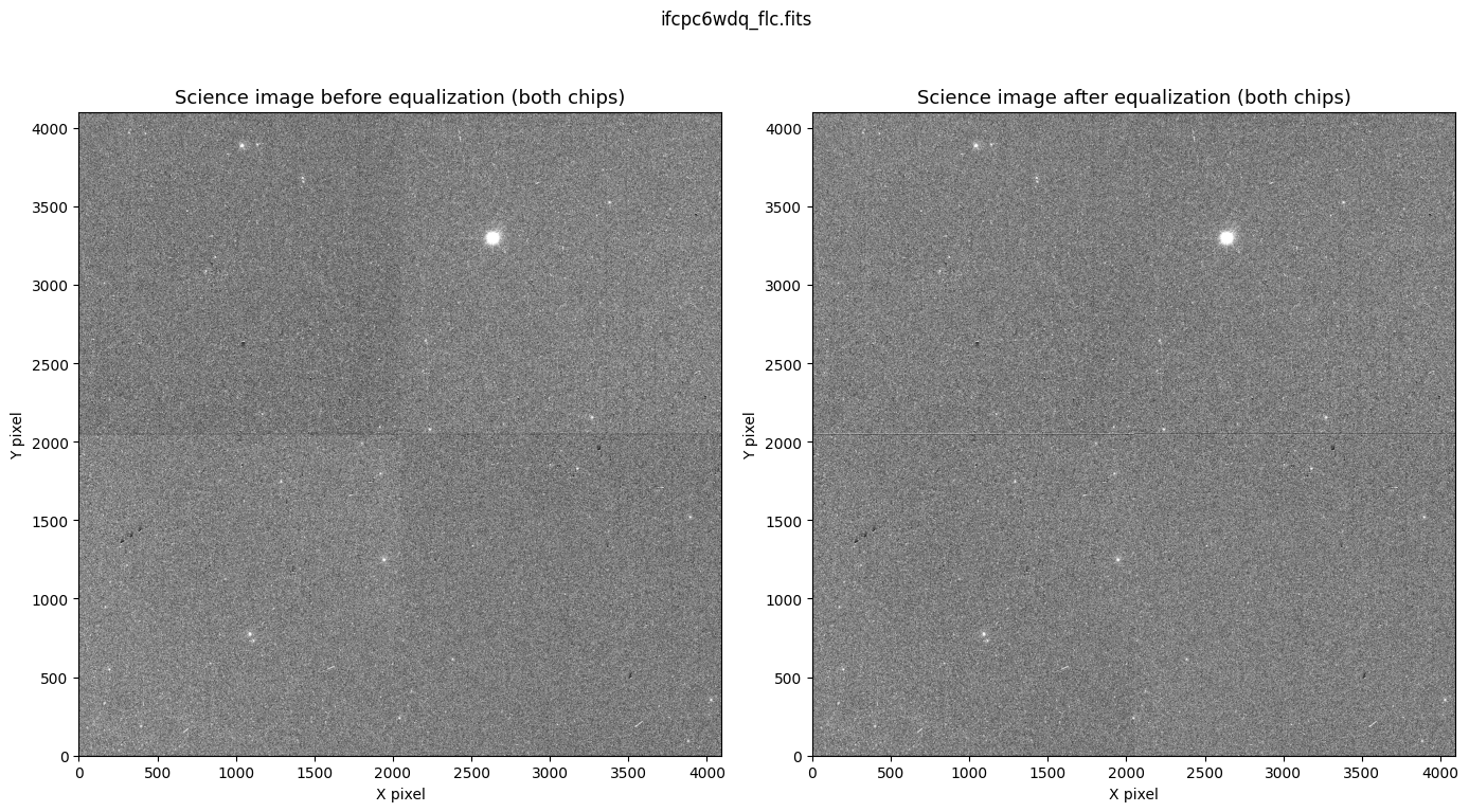
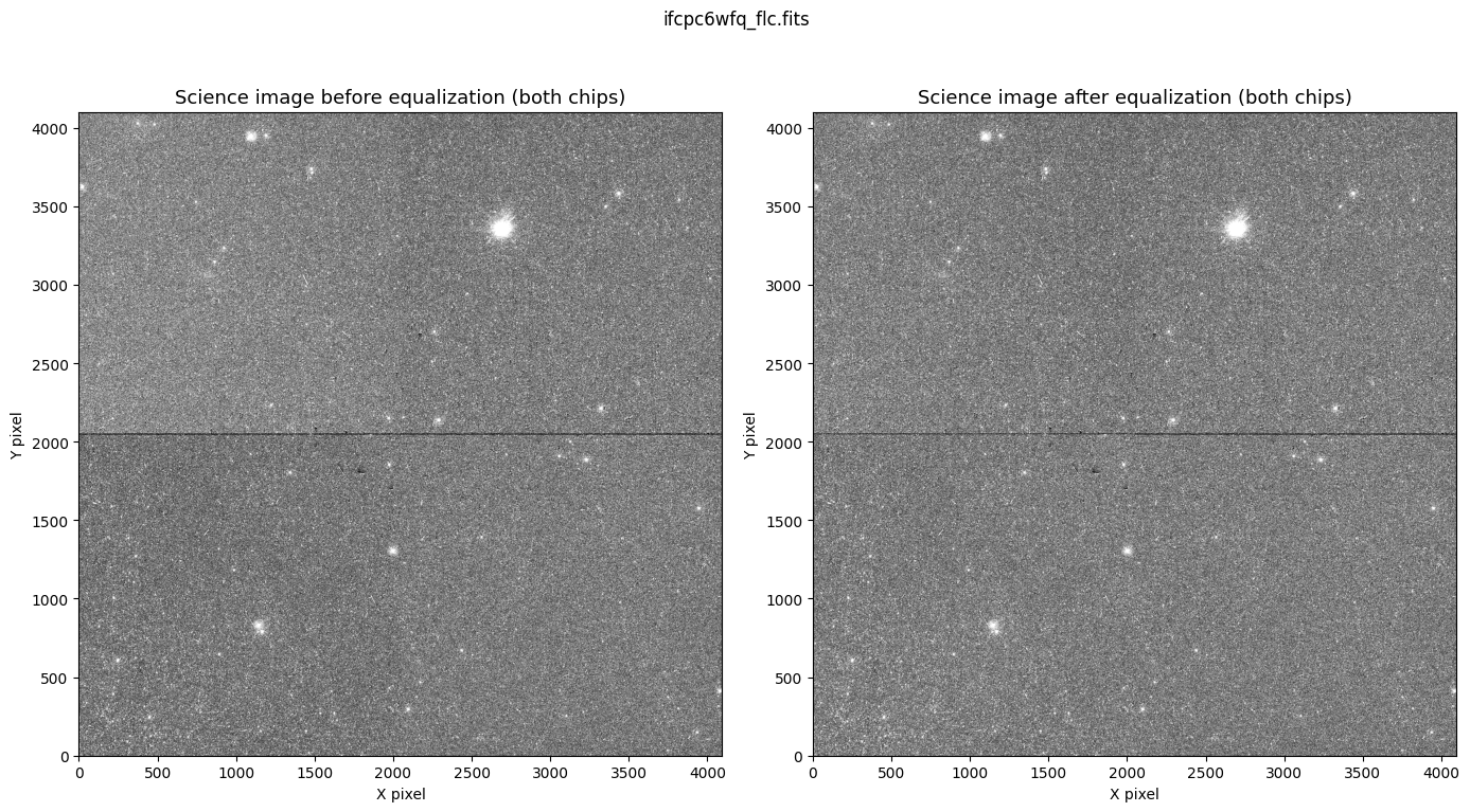
Below, we compare our original science data (left) and post-equalization science data (right) for each image. The science images after equalization no longer exhibit noticeable amp-to-amp brightness differences, as their background levels differ by only a fraction of an electron.

# Full image comparison before and after equalization
for fname in files:
    example_file = fname
    example_eq_file = example_file.replace('.fits', '_eq.fits')

    # Load both chips
    data_ext1 = fits.getdata(example_file, 1)  # UVIS2
    data_ext4 = fits.getdata(example_file, 4)  # UVIS1

    data_eq_ext1 = fits.getdata(example_eq_file, 1)
    data_eq_ext4 = fits.getdata(example_eq_file, 4)

    # Stack vertically
    data_full = np.vstack([data_ext1, data_ext4])
    data_eq_full = np.vstack([data_eq_ext1, data_eq_ext4])

    vmin, vmax = np.percentile(data_full, [49, 51])

    fig, axes = plt.subplots(1, 2, figsize=(14, 8))

    axes[0].imshow(data_full, origin='lower', cmap='gray', vmin=vmin, vmax=vmax)
    axes[0].set_title('Science image before equalization (both chips)', fontsize=13)
    axes[0].set_xlabel('X pixel')
    axes[0].set_ylabel('Y pixel')

    axes[1].imshow(data_eq_full, origin='lower', cmap='gray', vmin=vmin, vmax=vmax)
    axes[1].set_title('Science image after equalization (both chips)', fontsize=13)
    axes[1].set_xlabel('X pixel')
    axes[1].set_ylabel('Y pixel')

    plt.suptitle(os.path.basename(example_file), fontsize=12)
    plt.tight_layout()
    plt.show()

10. Step 6 — Re-Drizzle the Corrected Images

If you downloaded a pre-drizzled DRZ or DRC product and only applied amp equalization to the underlying FLT/FLCs, you must re-drizzle, as the downloaded DRZ/DRC was created from the uncorrected frames and will not reflect your changes. If you are starting fresh from FLT/FLC and have not yet drizzled, simply run AstroDrizzle on the *_eq.fits files directly. The corrected *_eq.fits images can be combined into a drizzled image using AstroDrizzle from the drizzlepac package.

We provide a worked example using our 2 example images below; see the DrizzlePac handbook and the DrizzlePac notebooks for full guidance on parameters.

tweakreg.TweakReg(
    eq_files,
    imagefindcfg={"threshold": 200, "conv_width": 6},
    shiftfile=True,
    outshifts="shift_equalized_flc_test.txt",
    wcsname='TWEAK1',
    updatehdr=True,
    interactive=False,
    ylimit=0.4,
    searchrad=0.15,
    tolerance=1
)

Setting up logfile :  tweakreg.log

TweakReg Version 3.10.0 started at: 21:31:48.463 (21/07/2026) 

Version Information

--------------------

Python Version 3.12.13 | packaged by conda-forge | (main, Mar  5 2026, 16:50:00) [GCC 14.3.0]

numpy Version -> 2.2.6 

astropy Version -> 7.1.0 

stwcs Version -> 1.7.7 

photutils Version -> 2.3.0 

Finding shifts for: 

    ifcpc6wdq_flc_eq.fits

    ifcpc6wfq_flc_eq.fits

===  Source finding for image 'ifcpc6wdq_flc_eq.fits':

  #  Source finding for 'ifcpc6wdq_flc_eq.fits', EXT=('SCI', 1) started at: 21:31:48.598 (21/07/2026)

     Found 3677 objects.

  #  Source finding for 'ifcpc6wdq_flc_eq.fits', EXT=('SCI', 2) started at: 21:31:49.192 (21/07/2026)

     Found 3970 objects.

===  FINAL number of objects in image 'ifcpc6wdq_flc_eq.fits': 7647

===  Source finding for image 'ifcpc6wfq_flc_eq.fits':

  #  Source finding for 'ifcpc6wfq_flc_eq.fits', EXT=('SCI', 1) started at: 21:31:50.184 (21/07/2026)

     Found 4492 objects.

  #  Source finding for 'ifcpc6wfq_flc_eq.fits', EXT=('SCI', 2) started at: 21:31:50.801 (21/07/2026)

     Found 4785 objects.

===  FINAL number of objects in image 'ifcpc6wfq_flc_eq.fits': 9277

===============================================================

Performing alignment in the projection plane defined by the WCS

derived from 'ifcpc6wdq_flc_eq.fits'

===============================================================

====================

Performing fit for: ifcpc6wfq_flc_eq.fits

Matching sources from 'ifcpc6wfq_flc_eq.fits' with sources from reference image 'ifcpc6wdq_flc_eq.fits'

Computing initial guess for X and Y shifts...

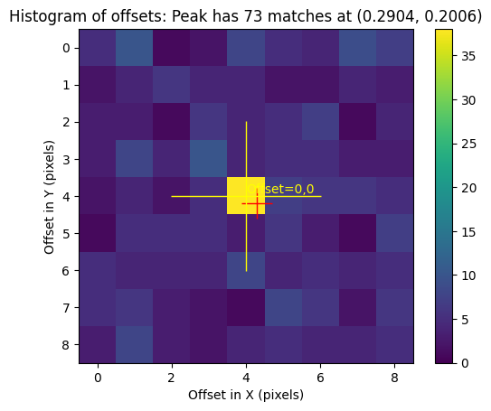
Found initial X and Y shifts of 0.2904, 0.2006 with significance of 34.7 and 191 matches

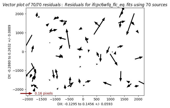
Found 84 matches for ifcpc6wfq_flc_eq.fits...

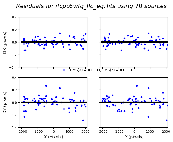
Computed  rscale  fit for  ifcpc6wfq_flc_eq.fits : 

XSH: 0.0068  YSH: 0.0762    ROT: 359.9974757    SCALE: 0.999985

FIT XRMS: 0.059      FIT YRMS: 0.088  

FIT RMSE: 0.11       FIT MAE: 0.086  

RMS_RA: 1.2e-06 (deg)   RMS_DEC: 1.3e-07 (deg)

Final solution based on  70  objects.

wrote XY data to:  ifcpc6wfq_flc_eq_catalog_fit.match

Total # points: 70

# of points after clipping: 70

Total # points: 70

# of points after clipping: 70

....Updating header for 'ifcpc6wfq_flc_eq.fits' ...

Processing ifcpc6wfq_flc_eq.fits['SCI',1]

Updating header for ifcpc6wfq_flc_eq.fits[1]

WCS Keywords

CD_11  CD_12: np.float64(7.599778331100951e-06) np.float64(8.51245464635599e-06)

CD_21  CD_22: np.float64(8.051408261699605e-06) np.float64(-7.074823043756955e-06)

CRVAL    : np.float64(296.2682869275278) np.float64(-14.775977755026622)

CRPIX    : np.float64(2048.0) np.float64(1026.0)

NAXIS    : 4096 2051

Plate Scale : np.float64(0.03985740704108994)

ORIENTAT : np.float64(129.73045601315368)

WCSNAME  :  TWEAK1

Processing ifcpc6wfq_flc_eq.fits['SCI',2]

Updating header for ifcpc6wfq_flc_eq.fits[4]

WCS Keywords

CD_11  CD_12: np.float64(7.608563834297498e-06) np.float64(8.404399141605136e-06)

CD_21  CD_22: np.float64(7.958447017061241e-06) np.float64(-7.000260882056069e-06)

CRVAL    : np.float64(296.2864949294335) np.float64(-14.790637684208956)

CRPIX    : np.float64(2048.0) np.float64(1026.0)

NAXIS    : 4096 2051

Plate Scale : np.float64(0.03963655793466246)

ORIENTAT : np.float64(129.79186855104592)

WCSNAME  :  TWEAK1

Processing ifcpc6wdq_flc_eq.fits['SCI',1]

Updating header for ifcpc6wdq_flc_eq.fits[('SCI', 1)]

WCS Keywords

CD_11  CD_12: np.float64(7.5991865835692e-06) np.float64(8.5132005664024e-06)

CD_21  CD_22: np.float64(8.0520637738346e-06) np.float64(-7.0742977570055e-06)

CRVAL    : np.float64(296.26921308347) np.float64(-14.775948650781)

CRPIX    : np.float64(2048.0) np.float64(1026.0)

NAXIS    : 4096 2051

Plate Scale : np.float64(0.039858254427877014)

ORIENTAT : np.float64(129.72589698635753)

WCSNAME  :  TWEAK1

Processing ifcpc6wdq_flc_eq.fits['SCI',2]

Updating header for ifcpc6wdq_flc_eq.fits[('SCI', 2)]

WCS Keywords

CD_11  CD_12: np.float64(7.6079803306179e-06) np.float64(8.4051370275424e-06)

CD_21  CD_22: np.float64(7.959102005438e-06) np.float64(-6.9997424321192e-06)

CRVAL    : np.float64(296.28742268104) np.float64(-14.79060749394)

CRPIX    : np.float64(2048.0) np.float64(1026.0)

NAXIS    : 4096 2051

Plate Scale : np.float64(0.039637400974265546)

ORIENTAT : np.float64(129.78730814302136)

WCSNAME  :  TWEAK1

Writing out shiftfile : shift_equalized_flc_test.txt

Trailer file written to:  tweakreg.log

# The following lines of code find and download the MDRIZTAB reference file which can be used as drizzle parameters
mdz = fits.getval(eq_files[0], 'MDRIZTAB', ext=0).split('$')[1]
print('Searching for the MDRIZTAB file:', mdz)
os.system(f'crds sync --hst --files {mdz} --output-dir {os.environ["iref"]}')

Searching for the MDRIZTAB file: 2ck18260i_mdz.fits

CRDS - INFO -  Symbolic context 'hst-latest' resolves to 'hst_1345.pmap'
CRDS - INFO -  Reorganizing 0 references from 'instrument' to 'flat'
CRDS - INFO -  Reorganizing from 'instrument' to 'flat' cache,  removing instrument directories.
CRDS - INFO -  Syncing explicitly listed files.
CRDS - INFO -  0 errors
CRDS - INFO -  0 warnings
CRDS - INFO -  4 infos

0

def get_vals_from_mdriztab(
    input_files,
    kw_list=[
        "driz_sep_bits",
        "combine_type",
        "driz_cr_snr",
        "driz_cr_scale",
        "final_bits",
    ],
):
    """Get only selected parameters from. the MDRIZTAB"""
    mdriz_dict = getMdriztabPars(input_files)

    requested_params = {}

    print("Outputting the following parameters:")
    for k in kw_list:
        requested_params[k] = mdriz_dict[k]
        print(k, mdriz_dict[k])

    return requested_params


selected_params = get_vals_from_mdriztab(eq_files)

- MDRIZTAB: AstroDrizzle parameters read from row 2.
Outputting the following parameters:
driz_sep_bits 336
combine_type minmed
driz_cr_snr 3.5 3.0
driz_cr_scale 1.5 1.2
final_bits 336

output_name = 'ifcpc6030_equalized'   # prefix for output DRZ file
astrodrizzle.AstroDrizzle(
    eq_files,
    output=output_name,
    **selected_params,
    preserve=False,
    clean=True,
    build=True,
    context=False,
    skymethod="match",
    runfile="f336w_eq_driz.log"
)

Setting up logfile :  f336w_eq_driz.log

AstroDrizzle log file: f336w_eq_driz.log

AstroDrizzle Version 3.10.0 started at: 21:32:03.384 (21/07/2026)

==== Processing Step  Initialization  started at  21:32:03.38 (21/07/2026)

WCS Keywords

Number of WCS axes: 2

CTYPE : 'RA---TAN' 'DEC--TAN' 

CRVAL : 296.27790486021956 -14.783278111398088 

CRPIX : 2090.0 2223.5 

CD1_1 CD1_2  : 7.071234826303351e-06 8.433261001397643e-06 

CD2_1 CD2_2  : 8.433261001397643e-06 -7.071234826303351e-06 

NAXIS : 4180  4447

********************************************************************************

*

*  Estimated memory usage:  up to 1107 Mb.

*  Output image size:       4180 X 4447 pixels. 

*  Output image file:       ~ 212 Mb. 

*  Cores available:         4

*

********************************************************************************

==== Processing Step Initialization finished at 21:32:04.036 (21/07/2026)

==== Processing Step  Static Mask  started at  21:32:04.038 (21/07/2026)

==== Processing Step Static Mask finished at 21:32:04.555 (21/07/2026)

==== Processing Step  Subtract Sky  started at  21:32:04.556 (21/07/2026)

***** skymatch started on 2026-07-21 21:32:04.662331

      Version 1.0.12

'skymatch' task will apply computed sky differences to input image file(s).

NOTE: Computed sky values WILL NOT be subtracted from image data ('subtractsky'=False).

'MDRIZSKY' header keyword will represent sky value *computed* from data.

-----  User specified keywords:  -----

       Sky Value Keyword:  'MDRIZSKY'

       Data Units Keyword: 'BUNIT'

-----  Input file list:  -----

   **  Input image: 'ifcpc6wdq_flc_eq.fits'

       EXT: 'SCI',1;	MASK: ifcpc6wdq_flc_skymatch_mask_sci1.fits[0]

       EXT: 'SCI',2;	MASK: ifcpc6wdq_flc_skymatch_mask_sci2.fits[0]

   **  Input image: 'ifcpc6wfq_flc_eq.fits'

       EXT: 'SCI',1;	MASK: ifcpc6wfq_flc_skymatch_mask_sci1.fits[0]

       EXT: 'SCI',2;	MASK: ifcpc6wfq_flc_skymatch_mask_sci2.fits[0]

-----  Sky statistics parameters:  -----

       statistics function: 'median'

       lower = None

       upper = None

       nclip = 5

       lsigma = 4.0

       usigma = 4.0

       binwidth = 0.1

-----  Data->Brightness conversion parameters for input files:  -----

   *   Image: ifcpc6wdq_flc_eq.fits

       EXT = 'SCI',1

             Data units type: COUNTS

             EXPTIME: 165.0 [s]

             Conversion factor (data->brightness):  3.860887199601451

       EXT = 'SCI',2

             Data units type: COUNTS

             EXPTIME: 165.0 [s]

             Conversion factor (data->brightness):  3.860887199601451

   *   Image: ifcpc6wfq_flc_eq.fits

       EXT = 'SCI',1

             Data units type: COUNTS

             EXPTIME: 700.0 [s]

             Conversion factor (data->brightness):  0.9100662684774848

       EXT = 'SCI',2

             Data units type: COUNTS

             EXPTIME: 700.0 [s]

             Conversion factor (data->brightness):  0.9100662684774848

***** skymatch started on 2026-07-21 21:32:04.820318

      Version 1.0.12

'skymatch' task will apply computed sky differences to input image file(s).

NOTE: Computed sky values WILL NOT be subtracted from image data ('subtractsky'=False).

'MDRIZSKY' header keyword will represent sky value *computed* from data.

-----  User specified keywords:  -----

       Sky Value Keyword:  'MDRIZSKY'

       Data Units Keyword: 'BUNIT'

-----  Input file list:  -----

   **  Input image: 'ifcpc6wdq_flc_eq.fits'

       EXT: 'SCI',1;	MASK: ifcpc6wdq_flc_skymatch_mask_sci1.fits[0]

       EXT: 'SCI',2;	MASK: ifcpc6wdq_flc_skymatch_mask_sci2.fits[0]

   **  Input image: 'ifcpc6wfq_flc_eq.fits'

       EXT: 'SCI',1;	MASK: ifcpc6wfq_flc_skymatch_mask_sci1.fits[0]

       EXT: 'SCI',2;	MASK: ifcpc6wfq_flc_skymatch_mask_sci2.fits[0]

-----  Sky statistics parameters:  -----

       statistics function: 'median'

       lower = None

       upper = None

       nclip = 5

       lsigma = 4.0

       usigma = 4.0

       binwidth = 0.1

-----  Data->Brightness conversion parameters for input files:  -----

   *   Image: ifcpc6wdq_flc_eq.fits

       EXT = 'SCI',1

             Data units type: COUNTS

             EXPTIME: 165.0 [s]

             Conversion factor (data->brightness):  3.860887199601451

       EXT = 'SCI',2

             Data units type: COUNTS

             EXPTIME: 165.0 [s]

             Conversion factor (data->brightness):  3.860887199601451

   *   Image: ifcpc6wfq_flc_eq.fits

       EXT = 'SCI',1

             Data units type: COUNTS

             EXPTIME: 700.0 [s]

             Conversion factor (data->brightness):  0.9100662684774848

       EXT = 'SCI',2

             Data units type: COUNTS

             EXPTIME: 700.0 [s]

             Conversion factor (data->brightness):  0.9100662684774848

-----  Computing sky values requested image extensions (detector chips):  -----

   *   Image:   'ifcpc6wdq_flc_eq.fits['SCI',1,2]'  --  SKY = 1.7793445587158203 (brightness units)

       Sky change (data units):

      - EXT = 'SCI',1   delta(MDRIZSKY) = 0.460864   NEW MDRIZSKY = 0.460864

      - EXT = 'SCI',2   delta(MDRIZSKY) = 0.460864   NEW MDRIZSKY = 0.460864

   *   Image:   'ifcpc6wfq_flc_eq.fits['SCI',1,2]'  --  SKY = 4.530864715576172 (brightness units)

       Sky change (data units):

      - EXT = 'SCI',1   delta(MDRIZSKY) = 4.97861   NEW MDRIZSKY = 4.97861

      - EXT = 'SCI',2   delta(MDRIZSKY) = 4.97861   NEW MDRIZSKY = 4.97861

***** skymatch ended on 2026-07-21 21:32:05.943887

TOTAL RUN TIME: 0:00:01.123569

==== Processing Step Subtract Sky finished at 21:32:05.947 (21/07/2026)

==== Processing Step  Separate Drizzle  started at  21:32:05.947 (21/07/2026)

WCS Keywords

Number of WCS axes: 2

CTYPE : 'RA---TAN' 'DEC--TAN' 

CRVAL : 296.27790486021956 -14.783278111398088 

CRPIX : 2090.0 2223.5 

CD1_1 CD1_2  : 7.071234826303351e-06 8.433261001397643e-06 

CD2_1 CD2_2  : 8.433261001397643e-06 -7.071234826303351e-06 

NAXIS : 4180  4447

-Generating simple FITS output: ifcpc6wdq_flc_eq_single_sci.fits

-Generating simple FITS output: ifcpc6wfq_flc_eq_single_sci.fits

Writing out image to disk: ifcpc6wdq_flc_eq_single_sci.fits

Writing out image to disk: ifcpc6wfq_flc_eq_single_sci.fits

Writing out image to disk: ifcpc6wdq_flc_eq_single_wht.fits

Writing out image to disk: ifcpc6wfq_flc_eq_single_wht.fits

==== Processing Step Separate Drizzle finished at 21:32:07.421 (21/07/2026)

==== Processing Step  Create Median  started at  21:32:07.423 (21/07/2026)

reference sky value for image 'ifcpc6wdq_flc_eq.fits' is 0.4608641564846039

reference sky value for image 'ifcpc6wfq_flc_eq.fits' is 4.978609561920166

Saving output median image to: 'ifcpc6030_equalized_med.fits'

==== Processing Step Create Median finished at 21:32:09.497 (21/07/2026)

==== Processing Step  Blot  started at  21:32:09.498 (21/07/2026)

    Blot: creating blotted image:  ifcpc6wdq_flc_eq.fits[sci,1]

Using default C-based coordinate transformation...

-Generating simple FITS output: ifcpc6wdq_flc_eq_sci1_blt.fits

Writing out image to disk: ifcpc6wdq_flc_eq_sci1_blt.fits

    Blot: creating blotted image:  ifcpc6wdq_flc_eq.fits[sci,2]

Using default C-based coordinate transformation...

-Generating simple FITS output: ifcpc6wdq_flc_eq_sci2_blt.fits

Writing out image to disk: ifcpc6wdq_flc_eq_sci2_blt.fits

    Blot: creating blotted image:  ifcpc6wfq_flc_eq.fits[sci,1]

Using default C-based coordinate transformation...

-Generating simple FITS output: ifcpc6wfq_flc_eq_sci1_blt.fits

Writing out image to disk: ifcpc6wfq_flc_eq_sci1_blt.fits

    Blot: creating blotted image:  ifcpc6wfq_flc_eq.fits[sci,2]

Using default C-based coordinate transformation...

-Generating simple FITS output: ifcpc6wfq_flc_eq_sci2_blt.fits

Writing out image to disk: ifcpc6wfq_flc_eq_sci2_blt.fits

==== Processing Step Blot finished at 21:32:13.840 (21/07/2026)

==== Processing Step  Driz_CR  started at  21:32:13.84 (21/07/2026)

Creating output: ifcpc6wdq_flc_eq_sci1_crmask.fits

Creating output: ifcpc6wfq_flc_eq_sci1_crmask.fits

Creating output: ifcpc6wdq_flc_eq_sci2_crmask.fits

Creating output: ifcpc6wfq_flc_eq_sci2_crmask.fits

==== Processing Step Driz_CR finished at 21:32:15.756 (21/07/2026)

==== Processing Step  Final Drizzle  started at  21:32:15.768 (21/07/2026)

WCS Keywords

Number of WCS axes: 2

CTYPE : 'RA---TAN' 'DEC--TAN' 

CRVAL : 296.27790486021956 -14.783278111398088 

CRPIX : 2090.0 2223.5 

CD1_1 CD1_2  : 7.071234826303351e-06 8.433261001397643e-06 

CD2_1 CD2_2  : 8.433261001397643e-06 -7.071234826303351e-06 

NAXIS : 4180  4447

-Generating multi-extension output file:  ifcpc6030_equalized_drz.fits

Deleted all instances of WCS with key A in extensions [1]

Deleted all instances of WCS with key B in extensions [1]

Deleted all instances of WCS with key C in extensions [1]

Writing out to disk: ifcpc6030_equalized_drz.fits

==== Processing Step Final Drizzle finished at 21:32:23.332 (21/07/2026)

AstroDrizzle Version 3.10.0 is finished processing at 21:32:23.333 (21/07/2026).

   --------------------          --------------------

                   Step          Elapsed time

   --------------------          --------------------

         Initialization          0.6500 sec.

            Static Mask          0.5177 sec.

           Subtract Sky          1.3905 sec.

       Separate Drizzle          1.4737 sec.

          Create Median          2.0742 sec.

                   Blot          4.3419 sec.

                Driz_CR          1.9153 sec.

          Final Drizzle          7.5641 sec.

   ====================          ====================

                  Total          19.9274 sec.

Trailer file written to:  f336w_eq_driz.log

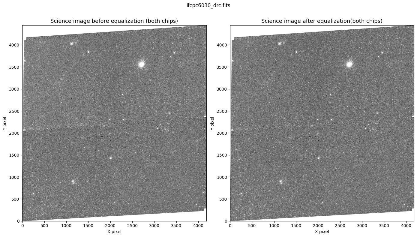
Finally, we plot the DRC science data (left) and new DRZ science data post-equalization (right) created by combining our images with Astrodrizzle. The new DRZ no longer has amp-to-amp brightness differences.

# Full drizzled image comparison before and after equalization

example_file = '../mastDownload/HST/ifcpc6030/ifcpc6030_drc.fits' 
example_eq_file = './ifcpc6030_equalized_drz.fits'

# Load drizzled images
data_full = fits.getdata(example_file, 1) 

data_eq_full = fits.getdata(example_eq_file, 1)

vmin, vmax = np.nanpercentile(data_full, [5, 95])

fig, axes = plt.subplots(1, 2, figsize=(14, 8))

axes[0].imshow(data_full, origin='lower', cmap='gray', vmin=vmin, vmax=vmax)
axes[0].set_title('Science image before equalization (both chips)', fontsize=13)
axes[0].set_xlabel('X pixel')
axes[0].set_ylabel('Y pixel')

axes[1].imshow(data_eq_full, origin='lower', cmap='gray', vmin=vmin, vmax=vmax)
axes[1].set_title('Science image after equalization(both chips)', fontsize=13)
axes[1].set_xlabel('X pixel')
axes[1].set_ylabel('Y pixel')

plt.suptitle(os.path.basename(example_file), fontsize=12)
plt.tight_layout()
plt.show()

11. Summary

Thank you for going through this notebook. You should now be familiar with the workflow to correct amp-dependent bias offsets in your WFC3 UVIS images, including the following steps:

• Downloading data from MAST.

• Measuring bias levels in each amp and computing individual offsets.

• Accounting for the flat-field.

• Equalizing amp-dependent bias levels across the image and redrizzling FLT/FLCs.

Additional Resources

Below are some additional resources that may be helpful. Please send any questions through the HST Help Desk.

• Sunnquist, B. 2019, UVIS Sky Darks, GitHub repository

• DrizzlePac documentation

• STScI HST Notebooks repository

About this Notebook

Author: Anne O’Connor, WFC3 Team

Created 2027-05-27

Citations

This notebook was developed based on the amp-equalization code and routines in:

Sunnquist, B. (2019). UVIS Sky Darks. GitHub. https://github.com/bsunnquist/uvis-skydarks

If you use this notebook in published work, please cite the original Sunnquist (2019) repository and any relevant Python packages such as astropy, astroquery, drizzlepac, matplotlib, or numpy. Follow these links for more information about citing various packages.

• Citing astropy

• Citing astroquery

• Citing drizzlepac

• Citing matplotlib

• Citing numpy

Top of Page